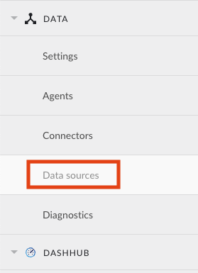
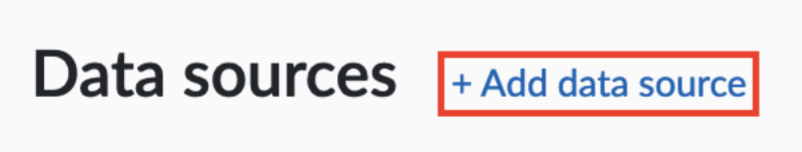
Data sources
When clicking on the Data sources menu option, the data sources overview is shown :
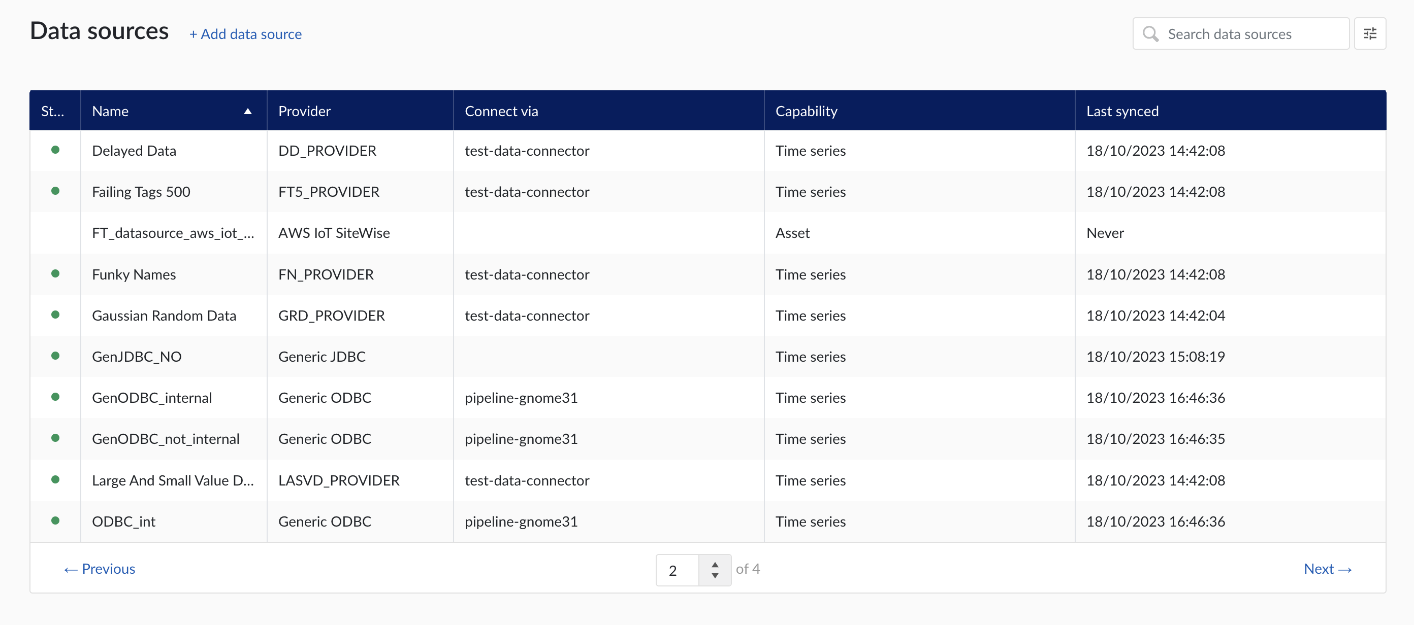
Data sources overview
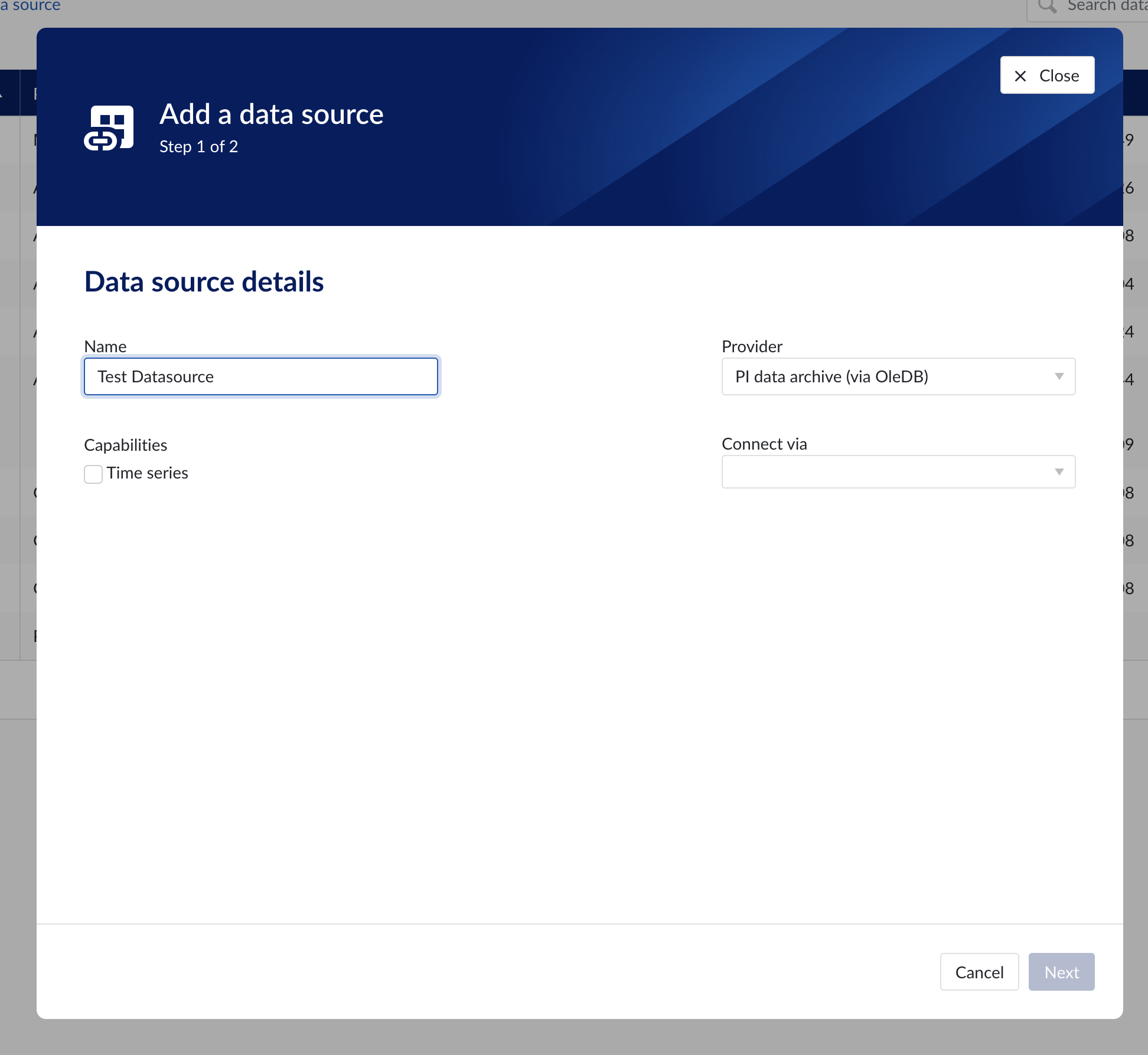
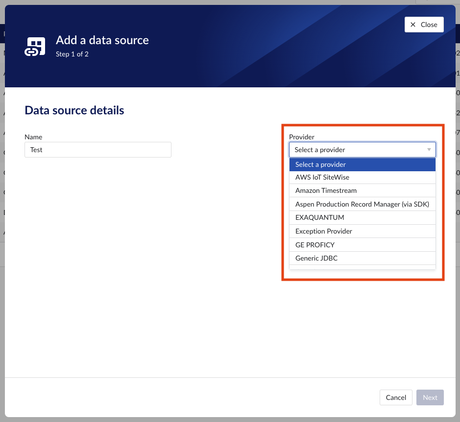
Add a new data source by clicking the (+ Add data source) label next to the title. An "Add a data source" modal will appear.
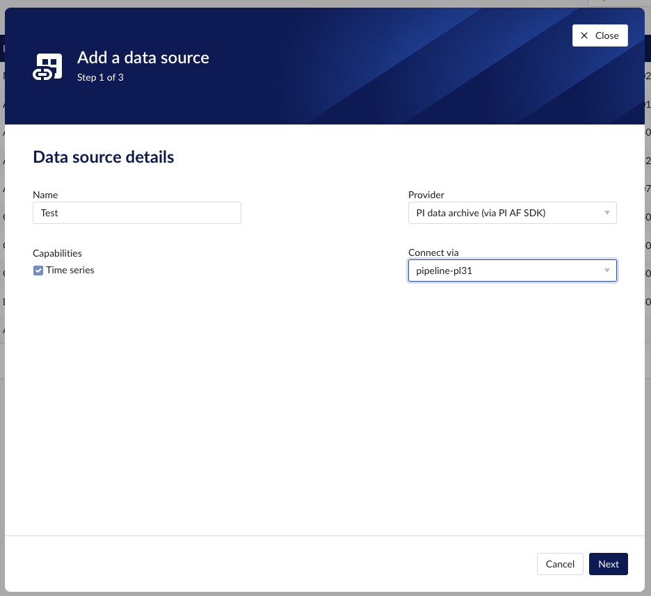
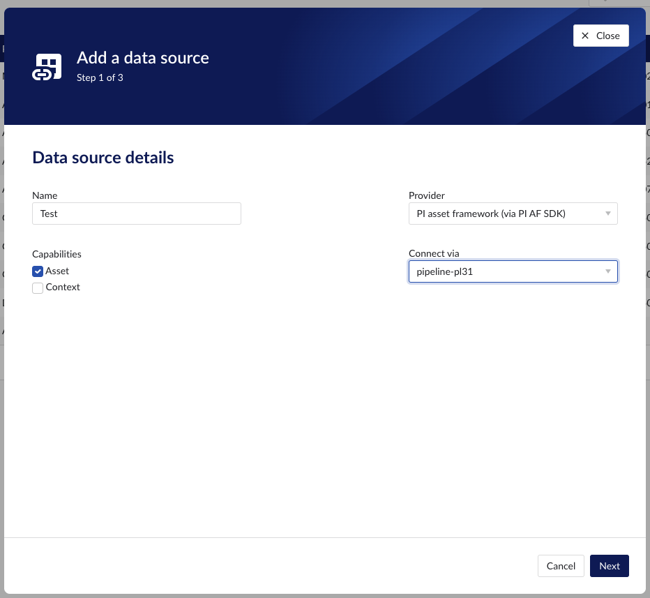
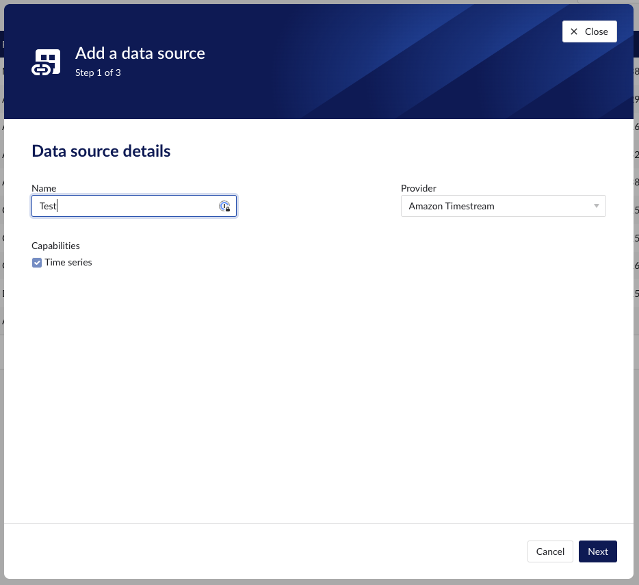
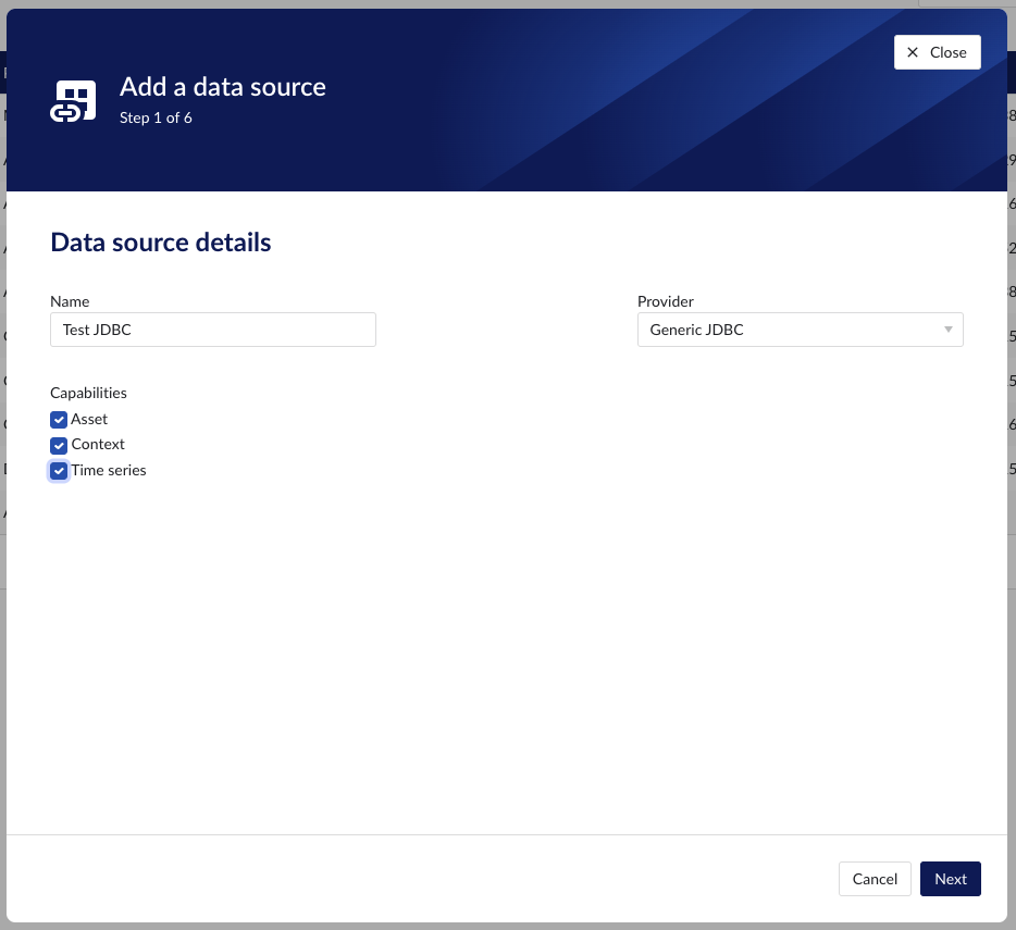
Data source details
Populate the fields on the Data source details step:
Name: you are free to choose data source names but they are mandatory, case insensitive and unique. The name of a data source identifies the data source. We strongly advise to only use alphanumerical and '-' or '_' in data source names as other characters are not supported in the access management so using special characters in a data source name might give issues when you want to assign access permission to the data source later on.
Provider: TrendMiner provides some out of the box connectivity to data sources via specific vendor implementations (e.g. OSIsoft PI, Honeywell PHD,...) and via more generic alternatives (e.g. Generic JDBC, ODBC, OleDB, ...). The provider 'TM connector' enables the connection of data sources via a connector to connector setup. To connect a data source via multiple connectors, extra configuration is needed via the TrendMiner Connector API.
Connect via: this dropdown is used to select a connector which is used to connect to the data source. The dropdown is displayed based on the selected provider: some data sources need to be connected via a connector (e.g. OSIsoft PI, Generic ODBC, Wonderware, ...), while others don't need any connector (e.g. Amazon Timestream, Generic JDBC, AWS IoT SiteWise, ...). To add a data source that needs a connector, the connector needs to be added first.
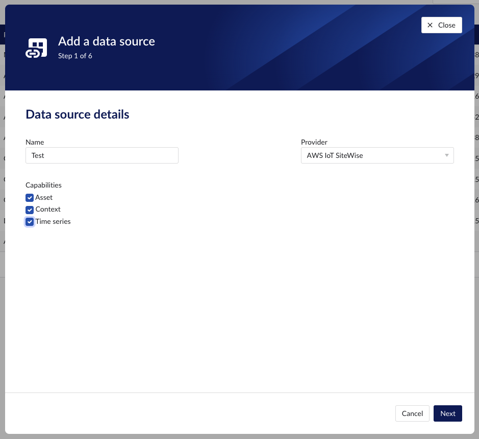
Capabilities: Capabilities depend on provider implementation. Some datasources have only one capability (e.g. Amazon Timestream has Time series capability only), others have all 3 capabilities (e.g. AWS IoT SiteWise). Selecting the capabilities for the data source with the given checkboxes will open additional properties to enter, grouped in following sections:
Connection details - lists properties related to the configuration of the connection that will be established with datasource
Time series details – lists properties relevant for the time series data
Asset details - lists properties relevant for asset data
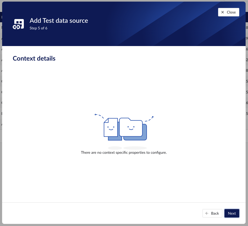
Context details - lists properties relevant for context data
Important
Duplicate tag names are not supported. If 2 tags with exactly the same name are synced to TrendMiner, analytics, calculations and indexing on/for these tags might fail. Use data source prefixes to avoid possible duplicate tag name issues.
Note
Depending on the provider you select, the connection details required for completion may differ.
Data source details step in the creation wizard
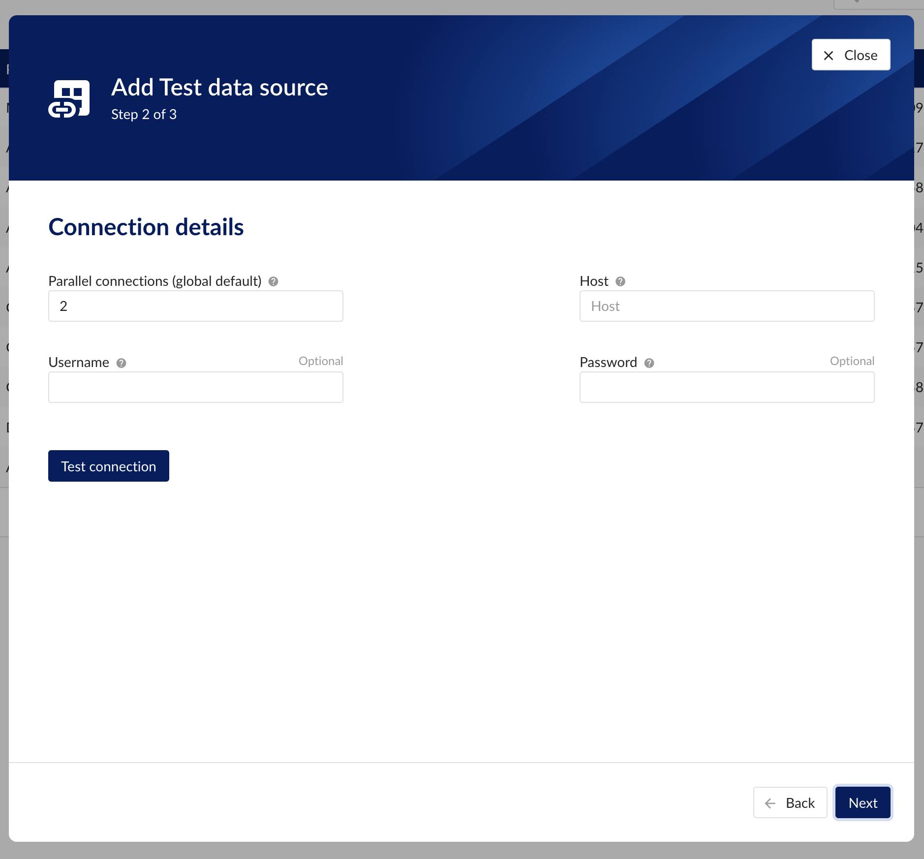
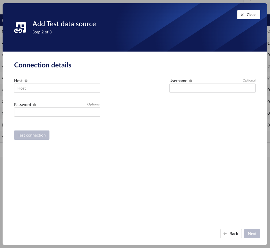
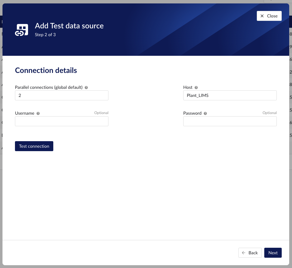
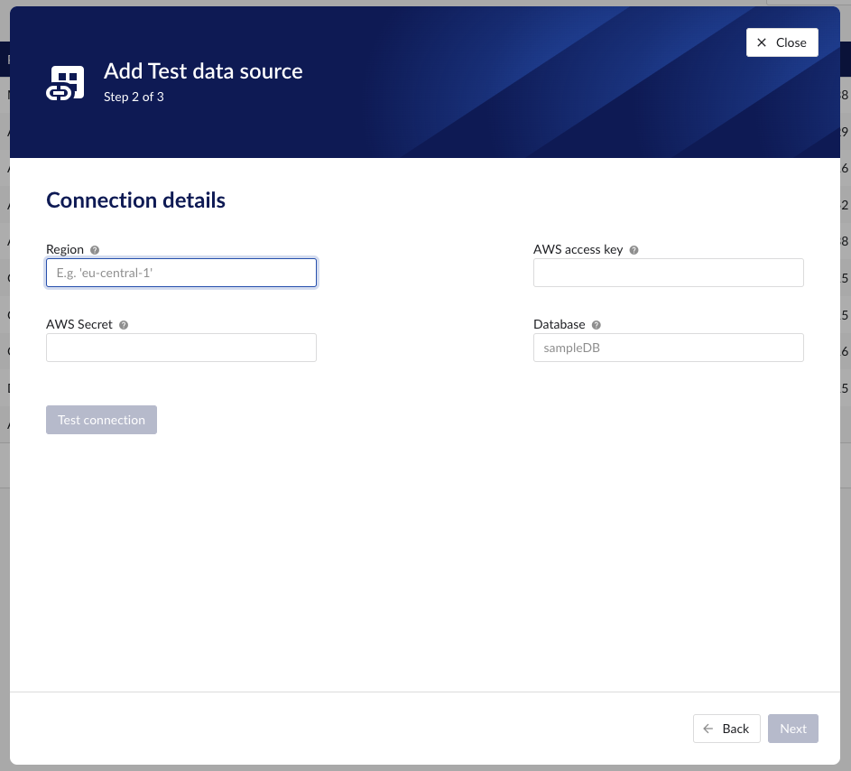
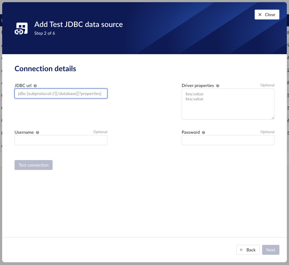
Connection details
Populate the fields on the Connection details step:
Parallel connections (if any): Each data source has 2 queues: one interactive - plot calls, one non-interactive - index calls, batch calls etc. Parallel connections determine how many connections each queue has to the connector. By default there are 2 parallel connections to the connector.
Host: the host name of the data source, e.g. myhistorian.mycompany.com
Username: username of the account configured in the data source.
Password: password of the account configured in the data source.
Once all mandatory fields are filled in, 'Test connection' button becomes enabled. By clicking on the button, user can verify the connection to the datasource.
Connection details step in the datasource creation wizard
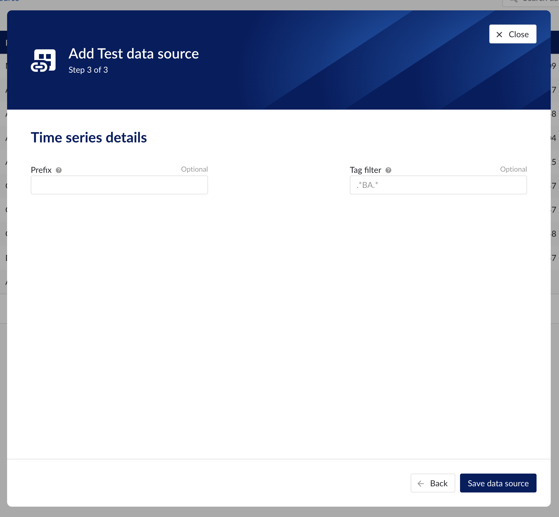
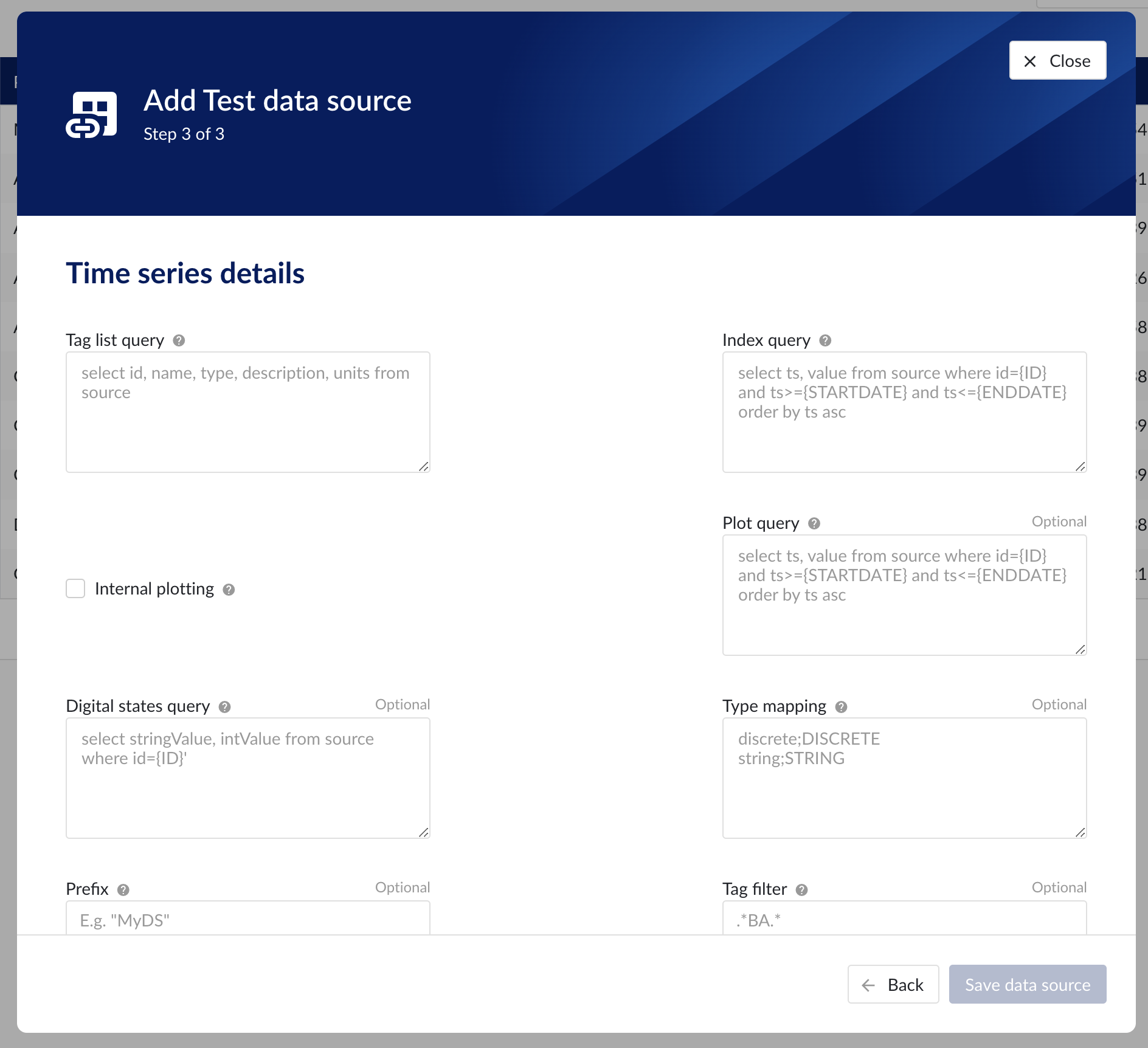
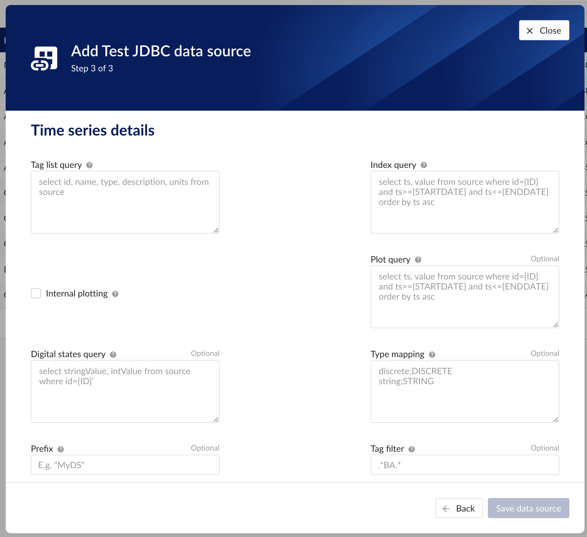
Time series details
Populate the fields on the Time series details step:
Prefix: you are free to choose prefixes. They are case insensitive but unique strings and have a maximum length of 5 characters. When synchronising a data source, all tag names of that data source will be prepended with the prefix to ensure tag name uniqueness in TrendMiner. Prefixes are optional but we highly recommend the provision of a prefix when connecting a data source to avoid duplicate tag names.
Tag filter: regular expression to be entered. Only tags with names that match this regular expression will be retained when creating tags (using the tag list query).
Examples:
Tag filter
Result
LINE.[1]+
Will make tags with 'LINE.1' in the name available but will exclude tags with 'LINE.3' in the tag name.
^(?:(?!BA:TEMP).).*$
Only excludes tag STARTING with BA:TEMP (so still keep test_BA:TEMP.1)
^\[pref\]PI.*$
Only syncs tags from a data source with prefix 'pref' and which start with 'PI'
Time series details step in the datasource creation wizard
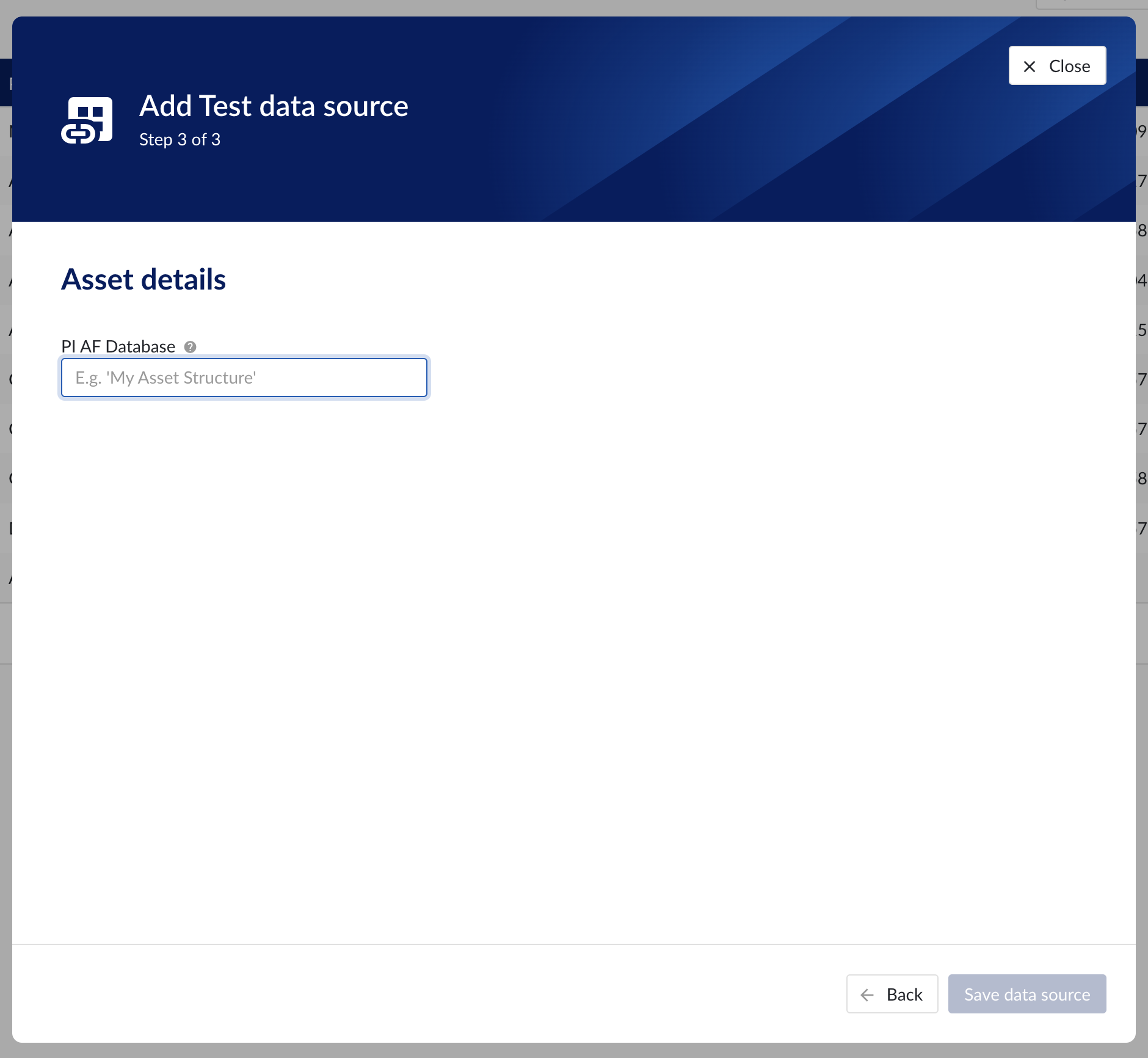
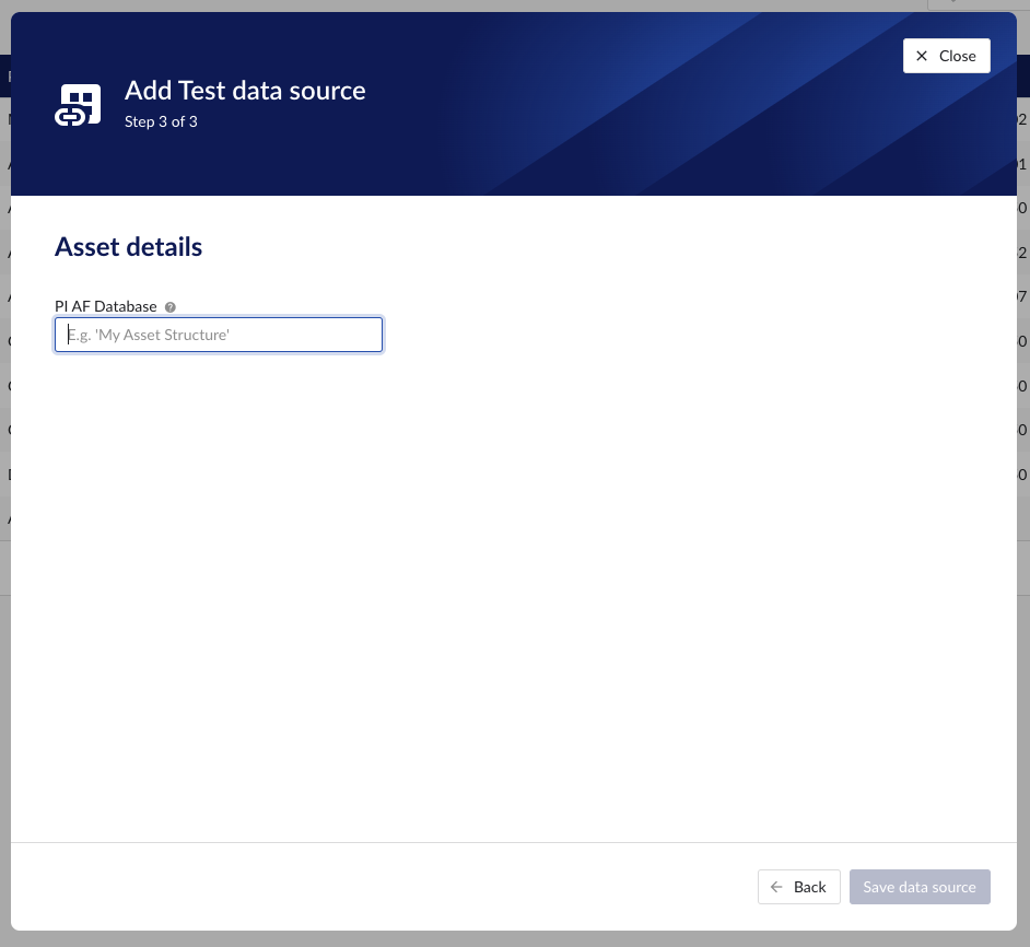
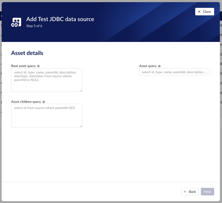
Asset details
The process of creating asset data source, is somewhat similar to the creation of time series data source, but fewer fields are required to fill in.
Database: name of the database to connect to.
Important
It is not permitted to add the same connection multiple times with asset capabilities enabled on both instances!
Asset tree permissions need to be managed in the asset permission section (ContextHub).
Asset details step in the datasource creation wizard
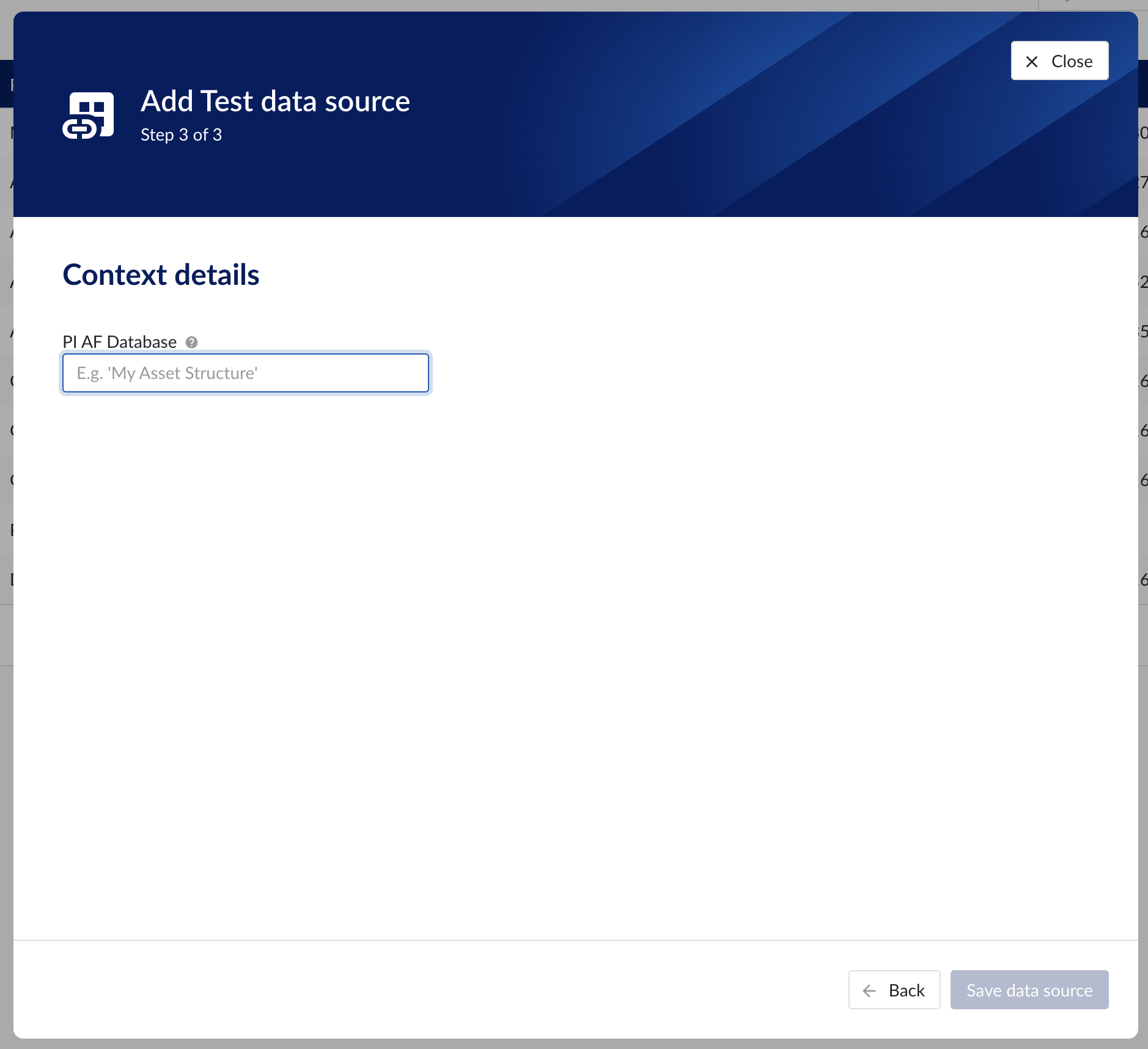
Context data
Context data sources are managed the same way as asset data sources. When a data source is context capable, the context capability checkbox can be checked, after which the correct database for context data needs to be specified.
Notice
Note
Context data synchronised from a data source in OSISoft PI will be related to asset data in TrendMiner based on the "referenced elements" on the PI event frames. The system will always attempt to relate the context item to the asset corresponding to the primary referenced element in PI (if it exists). Otherwise it will default to the first referenced element for which a corresponding asset is known in TrendMiner.
Important
It is not permitted to add the same connection multiple times with context capabilities enabled on both instances! This will result in the creation of duplicate context items.
Context details step in the datasource creation wizard
Data source menu
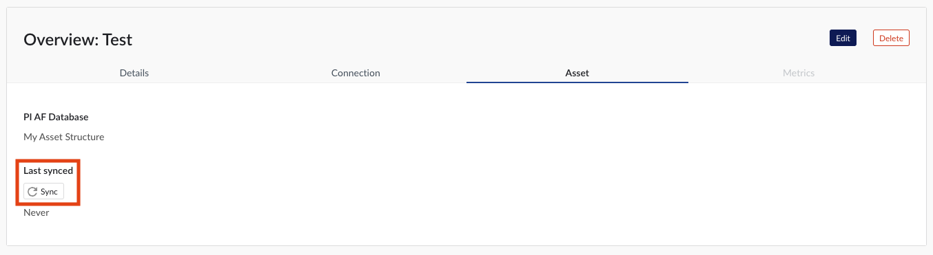
As soon as a new data source (with time series capability) is successfully added, it will start syncing all the tags from the data source, and can be found in the Data source overview.
To manually synchronise the data source, simply:
Click on the data source of your choice within the data source overview table. Datasource details will open below the datasources overview table.
Click on Time series tab.
Click on "Refresh tag cache" button.
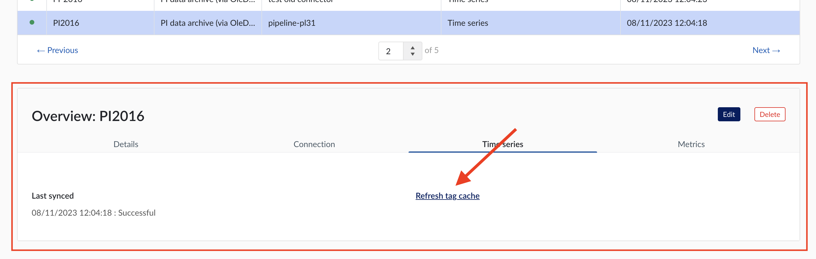
If a data source cannot be synced, the error feedback will be shown under 'Last synced' field.
For data sources which are successfully connected the 'Last synced' field in the data source details will show the last synced date and time and status 'Successful'. The last sync date and time will be updated when a manual sync is triggered or when TrendMiner synchronizes the tag cache for that data source, which happens automatically every 24 hours since the last refresh or service restart.
To edit the details of a data source, click on its name to open the datasource details tile below the overview table and then click on 'Edit' button. Datasource edit modal will appear.
It is prohibited to edit the prefix of an existing data source because it would break existing views, formulas, etc. All other fields can be updated after which the data source is synced again.
Other options available are:
Test connection (on Connection tab): this option will test the connection to the data source without triggering a sync and update the health status of the data source.
Delete: this option will remove the data source and all tags from this data source until it is connected again via a correctly configured connector.
When a data source is deleted, all tags from that data source will become unavailable immediately, as well as breaking views and calculations which depend on these tags. It is possible to restore these tags and dependent views and formulas by adding the data source again, using the exact same name and prefix via the same or alternate connector.
How to connect to time series data sources?
Install a connector. If your connector is already connected, this step can be skipped.
In ConfigHub select the tab "Connectors".
Click "+ Add connector" and fill in the details of the connector.
In ConfigHub select the tab "Data sources".
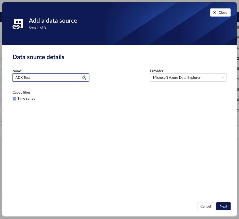
Click "+ Add data source". Datasource creation modal will appear.
Fill out 'Data source details' step:
Name the data source.
Select the provider you would like to use. If the provider of your choice is not listed, this implies none of the connected connectors supports this data source type and you have to add a connector which does, or check your implementation in case you implemented your own custom connector.
A list of providers which TrendMiner supports out of the box can be found here.
Select the connector you want to use for connecting the data source via 'Connect via' dropdown (if the provider of your choice requires a connector). If the connector of your choice is not listed, this implies this connector does not support this provider and you have to select a different connector or check your implementation in case you implemented your own custom connector.
Make sure to select the "Time series" capability checkbox. If this checkbox is not visible, it means this provider does not support time series data. You can check which connectivity options TrendMiner supports out of the box here.
Each data source with time series capability has some basic configuration options like "Host", "Username", "Password", "Parallel connections" etc. More information about these parameters can be found in our user documentation.
Besides the basic configuration each data source can have some historian specific configuration and installation requirements which can be found via the following links:
How to set up an Aveva PI AF data source?
Tip
To connect both time series and AF or EF data from an Aveva PI data source, 2 separate data sources need to be configured, one for the time series data and one for the AF and/or EF data.
Install the PI AF SDK 2017 or newer on the connector server.
Install a connector. If your connector is already connected this step can be skipped.
In ConfigHub select the tab "Connectors".
Click "+ Add connector" and fill in the details for the connector.
In ConfigHub select the tab "Data sources".
Click "+ Add data source". Data source creation modal will appear.
Fill out 'Data source details' step:
Name the data source.
Select the provider 'PI asset framework (via PI AF SDK)'.
Select the connector you want to use for connecting this data source via the 'Connect via' dropdown.
Make sure to select the "Asset" capability checkbox.
Fill out 'Connection details' step.
Fill out 'Asset details' step and click 'Save data source' button.
Newly created data sources can be reviewed in the overview section below the data sources grid. To sync the asset tree, click on 'Sync' button on Asset tab.
How to set up a Microsoft Azure Data Explorer data source?
The following sections will detail all the information needed for setting up a Microsoft Azure Data Explorer data source in TrendMiner.
Warning
The queries and examples on this page are for illustration only. Adjustments to fit your own specific environment may be required (e.g. matching data types) and fall outside of the scope of this support document.
If you wish to engage for hands-on support in setting up this connection, please reach out to your TrendMiner contact.
Danger
It is not recommended to use the "set notruncation;" option in your queries, as this will remove any restriction in the number of data points returned in each request. In extreme cases, this could cause TrendMiner services to run out of memory. It can be useful to add this option for initial testing, but do not use it in production to avoid sudden issues.
Note that, if a result set is truncated, Azure Data Explorer will return this query as FAILED and plotting/indexing on the TrendMiner side will also fail. This is to avoid working with incomplete data sets. If you run into the truncation limit regularly, it is advised to update your index granularity to a lower value. Also, ensure Analytics Optimization is implemented. An example is included in the next sections.
ConfigHub configuration
To add a Microsoft Azure Data Explorer data source, in ConfigHub go to Data in the left side menu, then Data sources, choose + Add data source.
Fill out 'Data source details' on the first step of the datasource creation wizard: type name of data source, select “Microsoft Azure Data Explorer” from the Provider dropdown. Time series capability will be checked by default.
Fill out additional properties, grouped in following sections:
Connection details – lists properties related to the configuration of the connection that will be established with Microsoft Azure Data Explorer.
Time series details – lists properties relevant for the time series data.
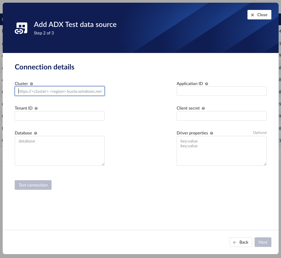
Following properties need to be populated to establish the connection:
“Name“ - а mandatory name needs to be specified.
“Provider” - select the option Microsoft Azure Data Explorer from the dropdown.
“Capabilities” - the only capability supported is the Time series capability. It will be selected by default.
“Prefix” - optional text can be entered here that will be used to prefix the tag names in TrendMiner, if a value is entered. Warning: this cannot be changed. The datasource can however be deleted and you can start the configuration over again.
"Cluster" - to be mapped with value of the cluster URI.
https://<cluster>.<region>.kusto.windows.net"Application ID" - a mandatory application id. In Azure a new application “TrendMiner” needs to be registered. After completion of this registration the application id will be available. For more info please refer to Azure Active Directory application registration or consult with the Azure Data Explorer documentation.
"Tenant ID" - a mandatory tenant id. In Azure a new application "TrendMiner"needs to be registered. After completion of this registration the tenant id is available.
"Client secret" - after registration of the TrendMiner application in Azure a client id and a secret need to be generated in order to get application access. The client secret for this access needs to be entered here.
"Database" – to be mapped with the name of the ADX database holding the time series data to be pulled.
"Driver properties" - additional optional driver specific properties can be configured here as key;value, where key is the name of driver specific property and value the desired value for this property.
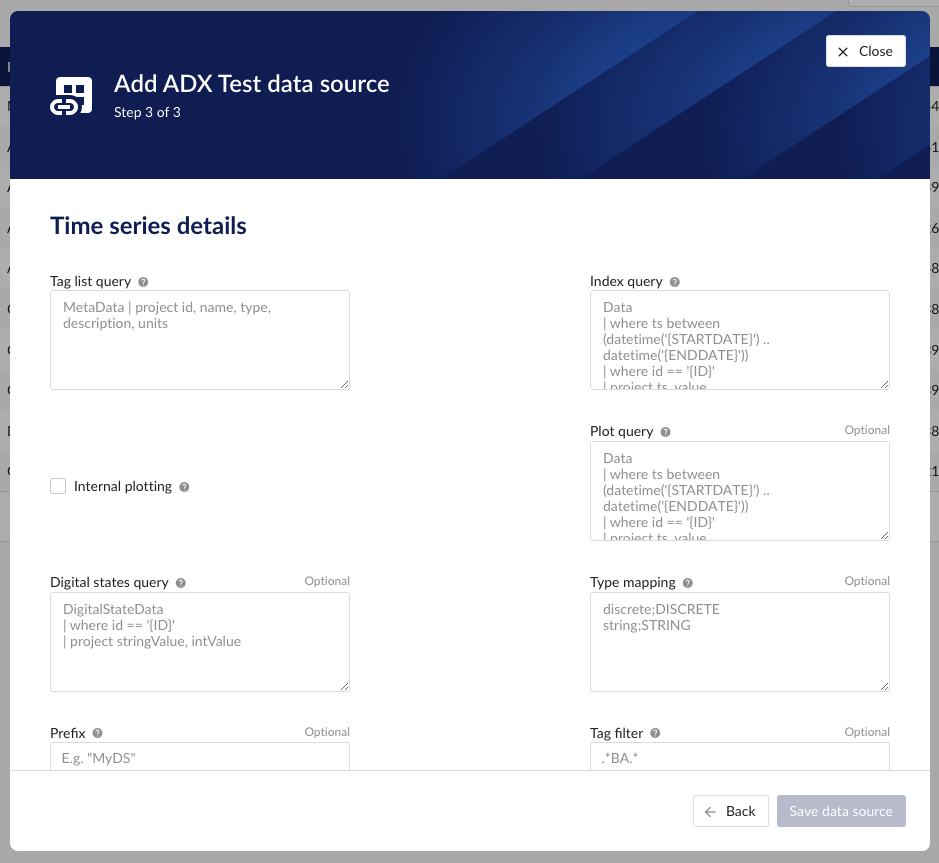
“Tag list query” - a query used by TrendMiner to create tags. A query needs to be provided that given the database schema and tables used will return the following columns:
id - this is mandatory and must have a unique value for each row returned by the query.
name - this is mandatory and must have a value.
type - an optional type indication. If the type column is not in the query, TrendMiner will use the default type which is ANALOG. Custom types can be returned here not known to TrendMiner but then a type mapping must be added as well. See also type mapping below. Without additional type mapping it must be one of the following TrendMiner tag types: ANALOG, DIGITAL, DISCRETE, STRING
description - an optional description to describe the tag. Can return an empty value or null.
units - an optional indication of the units of measurement for this tag. Can return an empty value or null.
The order of the columns in the query needs to be: id, name, type, description, units
“Index query” - a query used by TrendMiner to ingest timeseries data for a specific tag. The query is expected to return a ts (timestamp) and a value. The following variables are available to be used in the WHERE clause of this query. The variables will be substituted at query execution with values. There should not be any NULL values returned by the SELECT statement so including "IS NOT NULL" in the WHERE clause is strongly recommended.
{ID}. The id as returned by the tag list query.
{STARTDATE} TrendMiner will ingest data per intervals of time. This denotes the start of such an interval.
{ENDDATE} TrendMiner will ingest data per intervals of time. This denotes the end of such an interval.
{INTERPOLATION}: Interpolation type of a tag, which can be one of two values: LINEAR or STEPPED.
{INDEXRESOLUTION}: Index resolution in seconds. It can be used to optimise a query to return the expected number of points.
“Internal plotting” - if this option is selected TrendMiner will use interpolation if needed to plot the timeseries on the chart on specific time ranges. If this value is not selected and no plot query was provided, TrendMiner will plot directly from the index.
“Plot query” – a query used by TrendMiner to plot timeseries data for a specific tag. The query is expected to return a ts (timestamp) and a value. The following variables are available to be used in the WHERE clause of this query. The variables will be substituted at query execution with values. There should not be any NULL values returned by the SELECT statement so including "IS NOT NULL" in the WHERE clause is strongly recommended.
{ID}. The id as returned by the tag list query.
{STARTDATE}. TrendMiner will plot data per intervals of time. This denotes the start of such an interval.
{ENDDATE}. TrendMiner will plot data per intervals of time. This denotes the end of such an interval.
{INTERPOLATION}: Interpolation type of a tag, which can be one of two values: LINEAR or STEPPED.
{INDEXRESOLUTION}: Index resolution in seconds. It can be used to optimise a query to return the expected number of points.
“Digital states query” - if tags of type DIGITAL are returned by the tag list query, TrendMiner will use this query to ask for the {stringValue, intValue} pairs for a specific tag to match a label with a number. The query expects to return a stringValue and an intValue and can make use of the {ID} variable in the where clause. The variable will be substituted at query execution with a value.
“Tag filter” - an optional regular expression to be entered. Only tags with names that match this regex will be retained when creating tags (using the tag list query).
“Type mapping” - if types differ from what TrendMiner uses and one wants to avoid overcomplicating the query, a type mapping can be entered here. It can contain multiple lines and expect per line the value to be representing a custom type followed by a ; and a TrendMiner type. During the execution of the tag list query TrendMiner will then use this mapping to map the custom values returned in the query to TrendMiner tag types.
customTypeA;ANALOG
customTypeB;DIGITAL
customTypeC;DISCRETE
customTypeD;STRING
Example queries
Example 1 - Minimal configuration
This first example will only implement minimal logic to create a functioning data source. It will not consider Analytics Optimization or implement logic to handle different data types. It is recommended to start with this simple example to ensure the connectivity with ADX is functioning well and to check whether any constraints performance-wise would already pop up. Also, note that ADX will limit the number of output rows. This truncation default is typically 500,000 rows, but can be overridden. If the limit is hit however, ADX will consider this query as FAILED, which causes indexing in TrendMiner to stop.
To create a simple working set of tables with the schemas used in this documentation, the following queries can be executed. Note that this considers data entered as strings in the tables, even though they might represent numeric values (e.g. "5.01").
.create table MetaData (['id']: string, name: string, description: string, ['type']: string, units: string)
.create table Data (['id']: string, ts: datetime, value: string)
.create table DigitalStateData (['id']: string, intValue: long, stringValue: string)
Based on these tables, a tag list query to fetch all tags and their details is a simple project query.
MetaData | project id, name, type, description, units
The index query this simple example selects the data based on the parameters {ID}, {STARTDATE}, and {ENDDATE}. TrendMiner will fill in these variables when sending the query to ADX. Note that this query does not perform any analytics optimization or interpolation. It will simply return all rows that match the conditions. Due to the data schema (the value was defined as string type), this query works for ANALOG, DIGITAL, and STRING tags.
Data
| where ts between (datetime('{STARTDATE}') .. datetime('{ENDDATE}'))
| where id == '{ID}'
| project ts, value| order by ts asc
The plot query will be the same as the index query in this simple example. Once again, all rows that match the conditions will be returned without any further processing.
Data
| where ts between (datetime('{STARTDATE}') .. datetime('{ENDDATE}'))
| where id == '{ID}'
| project ts, value| order by ts asc
To map STRING values to a numeric value (to define the TrendHub y-axis plotting order), the following digital states query can be defined.
DigitalStateData
| where id == '{ID}'
| project stringValue, intValue
Example 2 - Extended configuration
This example will elaborate and will consider different datatypes in the queries and implement the Analytics Optimization. Note that implementing this in the query itself may come with a performance penalty as the logic needs to run when index data is fetched. Especially if the raw data contains many data points, it should be considered whether data can be pre-processed before it is fetched by TrendMiner.
The table schemas for this second example include one table (Data) for tags with decimal values and one table (StringData) for tags with non-decimal values.
.create table MetaData (['id']: string, name: string, description: string, ['type']: string, units: string)
.create table Data (['id']: string, ts: datetime, value: decimal)
.create table StringData ( ts: datetime, id: string, value: string)
.create table DigitalStateData (['id']: string, intValue: long, stringValue: string)
Based on these tables, same as above, a tag list query to fetch all tags and their details is a simple project query.
MetaData | project id, name, type, description, units
The index query in this example is a lot more complete as it handles different scenarios but at the cost of query complexity. Analytics optimization is implemented for numeric tags. This means numeric tags and non-numeric tags need to follow different query paths. This is done by using the union statement near the end of the query, which uses the output of the type filter to query the different tables.
let StringValuesQuery = view() {
    StringData
    | where id == '{ID}'
    | where ts between (datetime('{STARTDATE}') .. datetime('{ENDDATE}'))
    | order by ts asc
    | where isnotempty(value)
    | project ts, value
};
let NumericValuesQuery = view() {
    let _Data = Data
    | where id == '{ID}'
    | where ts between (datetime('{STARTDATE}') .. datetime('{ENDDATE}'))
    | where isnotempty(value)
    | project ts, value
    | order by ts asc;
    let MyTimeline = range ts from datetime('{STARTDATE}') to datetime('{ENDDATE}') step {INDEXRESOLUTION} * 1s;
    MyTimeline
    | union  withsource=source _Data
    | order by ts asc, source asc
    | serialize
    | scan declare (i_min:decimal, i_max:decimal, i_minTs:datetime, i_maxTs:datetime, startValue:decimal, endValue:decimal, startTs:datetime, endTs:datetime, min:decimal, minTs:datetime, max:decimal, maxTs: datetime) with
    (
        step s1 output=none: source=="union_arg0";
        step s2 output=none: source!="union_arg0"=> startValue = iff(isnull(s2.startValue), value, s2.startValue),
                                 startTs = iff(isnull(s2.startTs), ts, s2.startTs),
                                 i_min = iff(isnull(s2.i_min), value, iff(s2.i_min > value, value, s2.i_min)),
                                 i_minTs = iff(isnull(s2.i_min), ts, iff(s2.i_min > value, ts, s2.i_minTs)),
                                 i_max = iff(isnull(s2.i_max), value, iff(s2.i_max < value, value, s2.i_max)),
                                 i_maxTs = iff(isnull(s2.i_max), ts, iff(s2.i_max < value, ts, s2.i_maxTs));
        step s3 output=none: source!="union_arg0" => i_min = iff(isnull(s3.i_min), value, iff(s3.i_min > value, value, s3.i_min)),
                                 i_minTs = iff(isnull(s3.i_min), ts, iff(s3.i_min > value, ts, s3.i_minTs)),
                                 i_max = iff(isnull(s3.i_max), value, iff(s3.i_max < value, value, s3.i_max)),
                                 i_maxTs = iff(isnull(s3.i_max), ts, iff(s3.i_max < value, ts, s3.i_maxTs));
        step s4: source=="union_arg0" => startValue=s2.startValue,
                                     startTs=s2.startTs,
                                     min = s3.i_min,
                                     minTs = s3.i_minTs,
                                     max = s3.i_max,
                                     maxTs = s3.i_maxTs,
                                     endValue= s3.value,
                                     endTs= s3.ts;
    )
    | project startTs, startValue, endTs, endValue, minTs, min, maxTs, max
    | mv-expand     ts  = pack_array(startTs, minTs, maxTs, endTs) to typeof(datetime),
                value = pack_array(startValue, min, max, endValue) to typeof(string)
    | order by ts asc
    | where isnotempty(value)
    | project ts, value
};
let type = toscalar(MetaData
| where id == '{ID}'
| project type);
union (StringValuesQuery() | where tolower(type)=='string'), (NumericValuesQuery() | where not(tolower(type)=='string'))
| where isnotempty(value)
The plot query looks similar conceptually, but just returns raw data so is a lot shorter. Note again the conversion from decimal to string for the NumericValuesQuery to avoid a type mismatch in the union statement.
let StringValuesQuery = view() {
    StringData
    | where id == '{ID}'
    | where ts between (datetime('{STARTDATE}') .. datetime('{ENDDATE}'))
    | order by ts asc
    | where isnotempty(value)
    | project ts, value
};
let NumericValuesQuery = view() {
Data
  | where id == '{ID}'
  | where ts between (datetime('{STARTDATE}') .. datetime('{ENDDATE}'))
  | where isnotempty(value)
  | project ts, value=tostring(value)
  | order by ts asc;
};
let type = toscalar(MetaData
| where id == '{ID}'
| project type);
union (StringValuesQuery() | where tolower(type)=='string'), (NumericValuesQuery() | where not(tolower(type)=='string'))
| where isnotempty(value)
How to set up an ODBC/OLEDB/SQLite data source?
Notice
As of 2023.R4.0 TrendMiner supports an easier and better way to set up data sources via ODBC. This document describes the old way which is now considered deprecated.
If you want to set up a new connection via ODBC, please consider the Generic ODBC provider.
The following sections will detail all the information needed for setting up an ODBC/OLEDB/SQLite data source in TrendMiner.
Conventional SQL servers like MSSQL, MySQL, OracleDB, and others are all supported data sources that allow you to pull data into TrendMiner. It is important to know that process historians like Aveva PI, Wonderware and others might also support ODBC/OLEDB connectivity as their back-end databases are still SQL.
SQLite is a database engine that allows the creation of a file that serves as a relational database.
Overview
Configuring your SQL data source in TrendMiner requires these actions:
Plant Integration configuration on the connector side which consists of creating necessary files on a specific location.
Creation of specific queries and configuration elements that will fetch the data in the right format for TrendMiner to digest
Adding the data source on the client-side from the TrendMiner ConfigHub page.
Note
Ensure the correct drivers compatible with the data source you are attempting to connect to are installed on the Plant Integrations server. TrendMiner will use the driver as configured in the connection string (see below). Compatibility can be related to the version of the data source (e.g. version of MSSQL server), 32-bit or 64-bit, etc. Without a compatible driver, TrendMiner will not be able to successfully connect.
Plant integration configuration (Connector)
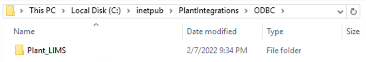
Create folders
First step is to browse to the Plant Integration folder you have created during installation. This folder will most likely reside inside the inetpub folder on the c drive of your connector server, which is the default location:
c:/inetpub/PlantIntegrations

Create a folder (not case sensitive) that will host all your ODBC/OLEDB/SQLite configuration files. All configuration files for ODBC connections will go into the ODBC folder, for OLEDB connections into the OLEDB folder and so on.
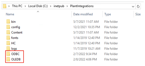
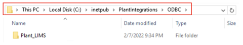
Create a subfolder for each data source you want to configure inside the correct ODBC/OLEDB/SQLite folder, depending on which connection type you are using. In the following example we will configure an ODBC data source called “Plant_LIMS”, so we create the "Plant_LIMS" subfolder in the recently created "ODBC" folder.
Create Configuration files
Create the following configuration files needed to configure the generic data sources.
For ODBC/OLEDB:
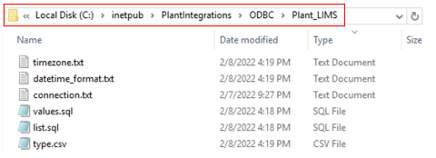
For SQLite:
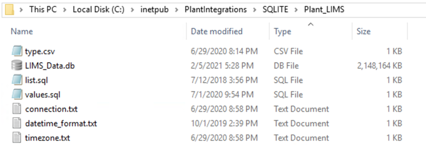
File name and type
Description
Required / Optional
sqlite.db (only for SQLite)
This is the sqlite.db file created that contains the data.
Required
connection.txt
Will contain the necessary information (e.g. full connection string) to establish the connection with the data source.
Required
list.sql
Query select statement that returns the list of tags with additional metadata.
Required
values.sql
Query select statement that returns the timestamps and values for a given tag.
Required
values-STRING.sql
Query select statement that returns the timestamps and values for a given string tag. Only include if necessary. If any string tags are not in the same database, you could use the query here or decide to join with your values.sql query.
Optional
type.csv
Specifies information for mapping all tag types available in the data source to those recognized by TrendMiner.
Required
datetime_format.txt
Specifies the date-time format of the timestamps returned by the values query
Optional
timezone.txt
Specifies the timezome associated to the timestamps if not already in UTC.
Optional
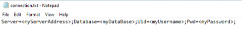
Connection.txt file
The information provided to establish the connection with the data source can be provided as part of a full standalone connection string or by referencing a ‘data source’ already identified as a data source name using the ODBC drivers. Independent of the option that is chosen, the details should be added to the connection.txt file.
The following article contains additional information on the required format of a valid connection string and examples depending on the type of database being used:
https://www.connectionstrings.com/
Note that only one connection string is necessary to connect to a database. Different tables within one database will be accessible through the same connection.
Standalone Full Connection Strings
ODBC example:
Driver={ODBC Driver 13 for SQL Server};Server=<ipAddress,port>;Database=<database_name>;Uid=<myUsername>;Pwd=<myPassword>;Encrypt=yes;TrustServerCertificate=no;Connection Timeout=30;As a minimum requirement, you shall specify the Server, Database, Uid, and Pwd.
OLEDB example:
Provider=iHOLEDB.iHistorian.1;Persist Security Info=False;USER ID=<myUsername>;Password=<myPassword>; Data Source=<data source>;Mode=Read
SQLite example:
For SQLite, the connection string shall contain the full path to the sqlite.db file as shown below.
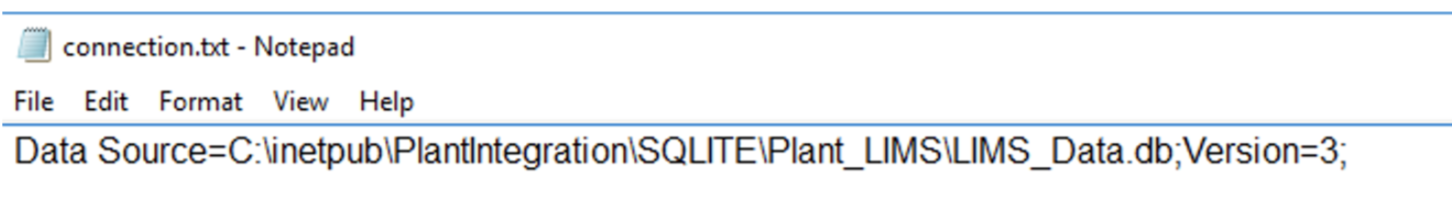 |
Connection via named data source using System ODBC drivers
Set up a new System Data Source using the corresponding SQL Server driver.
Note
Make sure the username being used to access the SQL database has read access.
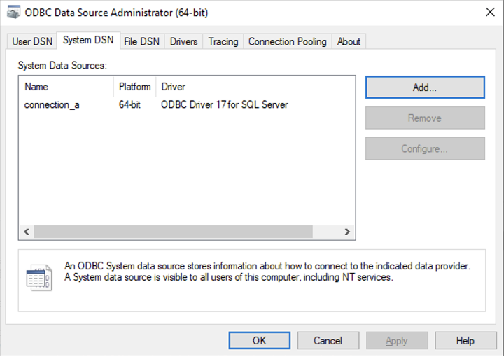
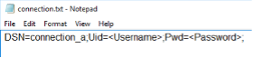
Once the System Data Source is configured, create a “connection.txt” file and make reference to the System Data Source as shown below.
Note
The username and password must be included in the file.
You can find additional information in the following article:
Configuring the queries
The data contained in your datasource now needs to be fetched in a way that TrendMiner can understand, to correctly digest and present back to the end users. There are a few steps required to make this work.
The first step is a query that will return unique tagnames (to identify the time series), its datatype, and optional metadata such as description and units. This query goes into the list.sql file.
The second step is a query that will return an ordered series of timestamp and value pairs for a given tagname, start date, and end date. This query goes into the values.sql file.
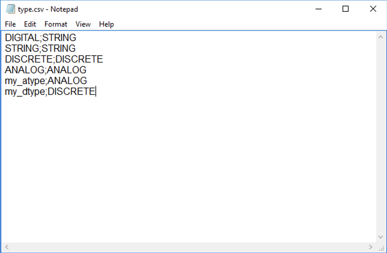
The third step is to map any custom datatypes to the TrendMiner datatypes. This mapping goes into the type.csv file.
The fourth step is to configure the returned timestamp format from step 2 so TrendMiner can parse it correctly. This step is optional and only required if the timestamp format returned in step 2 is not "yyyy-MM-dd HH:mm:ss.fff”
The fifth step is to configure the timezone of the returned timestamps from step 2 so TrendMiner can align it correctly. This step is optional and only required if the timestamps returned in step 2 are not in UTC. This is also important to correctly handle Daylight Savings Time (DST).
Details about all steps are documented in the sections below.
list.sql query
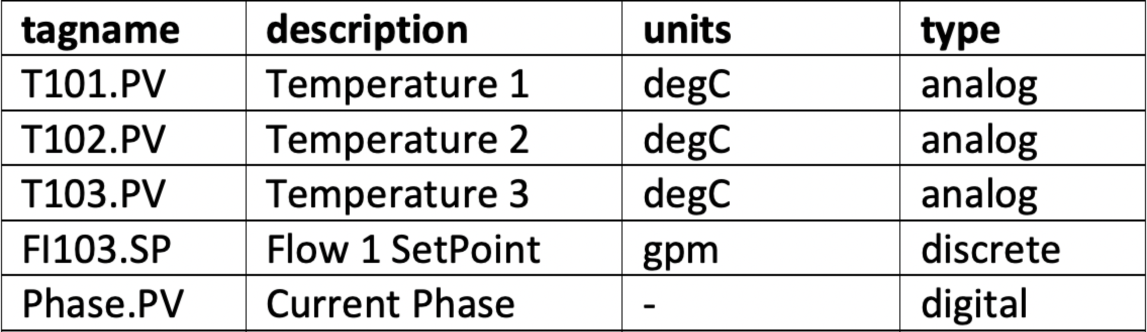
The list.sql file will contain a SQL SELECT statement and shall return all the tags with additional metadata as shown below. All your returned types should be mapped onto one of the supported tag types with the type.csv file.
The query should return a result with column names "tagname" (mandatory), "type" (mandatory), "units" (optional), and "description" (optional). All values for the tagnames returned by the query should be unique. Duplicates will lead to synch errors later on when connecting the datasource to TrendMiner in later steps. Stored procedures can be used for retrieving tags as long as they return a result set.
An example of a very simple query is given below. Note that the type has been hardcoded to be "analog". For additional examples, refer to the following article: Examples of SQL queries for ODBC connections.
SELECT
    tagname, description, units, "analog" as type
FROM Table_1
A correct output of the query is shown below:
values.sql query
The values.sql file will contain a SQL SELECT statement and shall return all the values and timestamps for a given tagname and date range. Note that these parameters (tagname, start date, and end date) will be automatically passed on by TrendMiner when in production as binding parameters.
These binding parameters are specified in the query by using question marks "?". If binding parameters (?) are not supported then .NET string formatting can be used, so use '{0}', '{1}', and '{2}' (include single quotes) instead of the question mark.
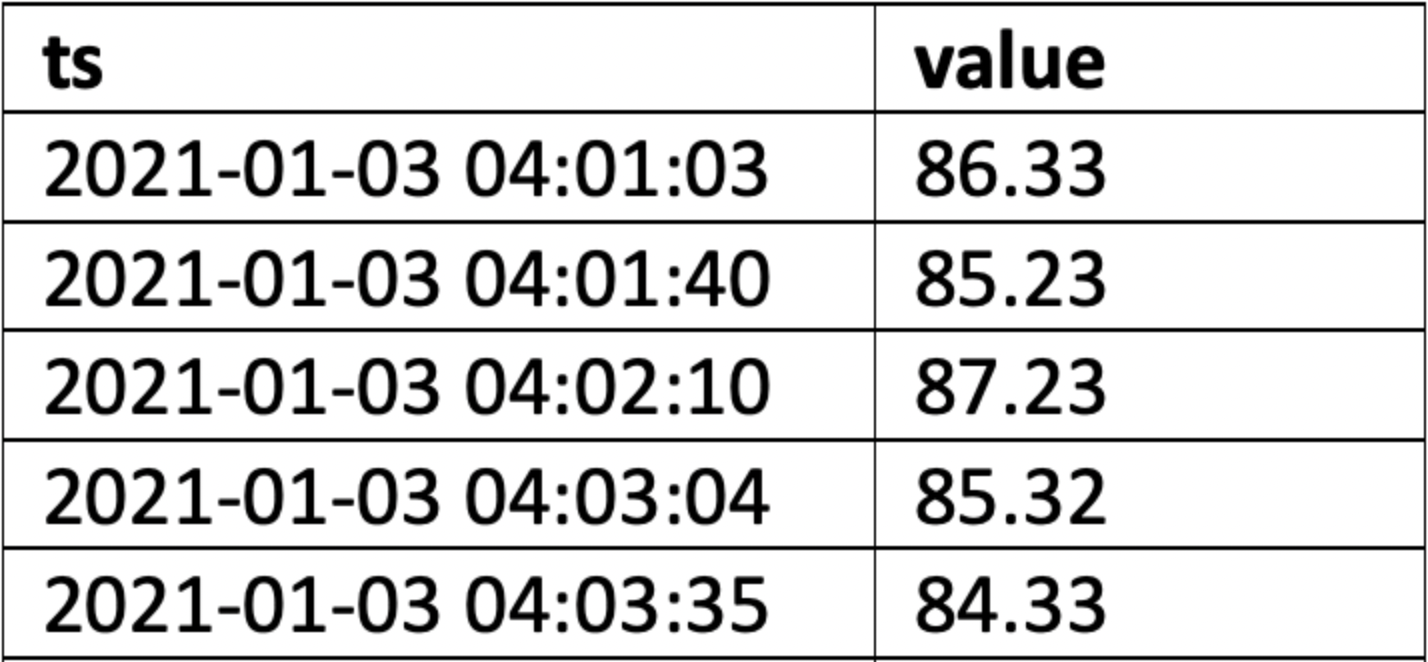
The query should return a result with column names "ts" (mandatory) and "value" (mandatory). The timestamps in the ts column should be ordered in ascending order (oldest point first, newest point last). Stored procedures can be used for retrieving tag data as long as they return a result set.
Since this is a crucial step, here is a summary of the output requirements:
The columns returned should be named "ts" (for the timestamp) and "value". Timestamps should be in ascending chronological order, meaning oldest first, newest last.
All timestamps that are returned should fall inside the requested time interval. If they don't, then indexing will fail later on.
The complete response should be returned within a reasonable timeframe. Typically recommended is +- 1 second per month of data, with user experience noticeably dropping off when response time exceeds 5 seconds per month of data. The response time can be influenced somewhat by tweaking settings such as the index granularity in ConfigHub, although a slow datasource will always lead to bottlenecks, no matter the settings. Check the user documentation for more info.
An acceptable amount of data points within the given timeframe. The number of data points returned can be influenced by tweaking the query, or by tweaking settings such as the index granularity setting in ConfigHub. Check the user documentation for more info.
An example of a simple query is given below. For additional examples, refer to the following article: Examples of SQL queries for ODBC connections.
SELECT
    ts, value
FROM Table_1
WHERE tagname = ? AND ts IS BETWEEN ? AND ? ORDER BY ts ASC
An example of the correct output is shown below.
 |
type.csv mapping
The types returned in the list.sql must be mapped to the types supported by TrendMiner, also if the returned type is the same as a TrendMiner supported type. You need to generate your own mapping. It is best practice to explicitly map each possible type returned by list.sql to one supported by TrendMiner. If no mapping/type.csv is provided all tags types will default to analog.
In the type.csv file, create one line per data type, with the output of the list.sql types as the first value, followed by a semicolon (";"), followed by one of the supported datatypes in TrendMiner. The example below ensures the results are returned in the right case, and a DIGITAL result is explicitly returned as a STRING result.
 |
datetime_format.txt configuration
In case the timestamps returned in the values.sql query are not in the format "yyyy-MM-dd HH:mm:ss.fff” (e.g. 2022-12-03 14:28:23.357), then the format can be configured by setting it in the datetime_format.txt file. Simply edit the txt file and paste the format in the file. The format is interpreted following the .NET formatting specification.
Alternatively, the file can contain the string “EPOCH”, in which case dates are converted to the equivalent number of seconds since the Epoch and the converted values are used in the query.
Some examples are specified below.
Without timezone (UTC) | MM/dd/yyy HH:mm |
DDMMYYY HH:mm:ss | |
With timezone | yyyy-MM-ddTHH:mm:ssZ |
yyyy-MM-ddTHH:mm:sszzz |
timezone.txt configuration
It is advised to always use timestamps in UTC. This will avoid confusion when troubleshooting, especially when datasources from different timezones are connected since TrendMiner uses UTC by default. If timestamps are stored in the datasource in local time, it is necessary to provide the timezone information.
Specify the time zone name in the timezone.txt file, using "Time zone name" as listed on https://docs.microsoft.com/en-us/previous-versions/windows/embedded/gg154758(v=winembedded.80).
Timezone |
|---|
Eastern Standard Time |
Pacific Standard Time |
Central Europe Standard Time |
Important
When the database stores date/times in a timezone which uses DST, but the timezone is not stored along with the date/time, then a 1 hour gap in the data will occur when entering summer time and 1 hour of data may be discarded when entering winter time.
Adding data source in ConfigHub
Follow the steps for adding a new data source as detailed in the user documentation.
The “Host” name will be the name of the folder previously created containing all the configuration files as in the example below. The data source name is free to choose.
TrendMiner will consider the username and password provided in the “connection.txt” file and not the one provided through the interface. You do not need to provide the username and password here.
More info
How to set up an AWS IoT SiteWise data source?
The following sections will detail all the information needed to set up an AWS IoT SiteWise data source in TrendMiner.
Communication flows
You can configure AWS IoT SiteWise to store data in following storage tiers: a hot tier optimized for real-time applications, and a cold tier optimized for analytical applications.
hot tier - a service-managed database. By default, your data is stored only in the hot tier of AWS IoT SiteWise. You can set a retention period for how long your data is stored in the hot tier before it's deleted. The hot tier can be queried through the AWS REST API.
cold tier – a customer-managed Amazon S3 bucket. AWS IoT SiteWise stores your data in an Amazon S3 bucket. You can use the cold tier to store historical data that requires infrequent access. Latency might be higher when you retrieve cold tier data. After your data is sent to the cold tier, you can use the Amazon Athena AWS service to run SQL queries on your data.
The cold tier requires additional configuration in AWS with regards to S3 and a Glue crawler. For more information about this, please consult the AWS documentation.
Setup an AWS IoT SiteWise data source
To add an AWS IoT SiteWise data source, in ConfigHub go to Data in the left side menu, then Data sources, choose + Add data source.
Fill out 'Data source details' on the first step of the datasource creation wizard: type name of data source, select “AWS IoT SiteWise” from the Provider dropdown.
Selecting the capabilities for the data source with the given checkboxes will open additional properties to enter, grouped in following sections:
Connection details – lists properties related to the configuration of the connection that will be established with AWS IoT SiteWise
Provider details - lists properties shared by multiple capabilities
Time series details– lists properties relevant for the time series data
Asset details – lists properties relevant for the asset data
Context details – lists properties relevant for the AWS IoT SiteWise alarms
Important
The time series storage in AWS IoT SiteWise is structured according to the asset hierarchy. No time series data can be obtained without first pulling the asset tree, and then based on it the time series data can be obtained.
As the time series and asset capabilities go hand in hand in AWS IoT SiteWise, the checkboxes for Asset and Time series capabilities must be selected together.
To pull AWS IoT SiteWise alarm data, select the Context capability checkbox.
Asset capability
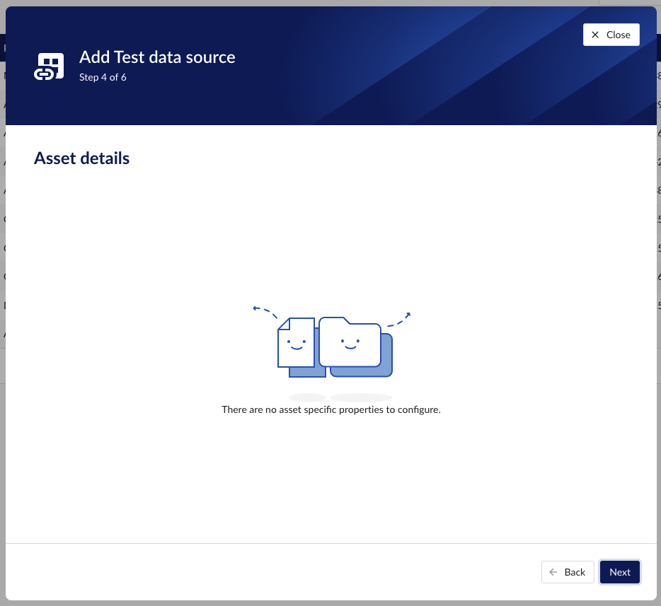
With this capability enabled the datasource can pull assets from AWS IoT SiteWise to be synced into a TrendMiner asset structure.
Following properties need to be populated:
“Name“ - а mandatory name needs to be specified.
“Provider” - select the option AWS IoT SiteWise from the dropdown.
“Capabilities” - the AWS IoT SiteWise provider supports Asset, Time series and Context capabilities.
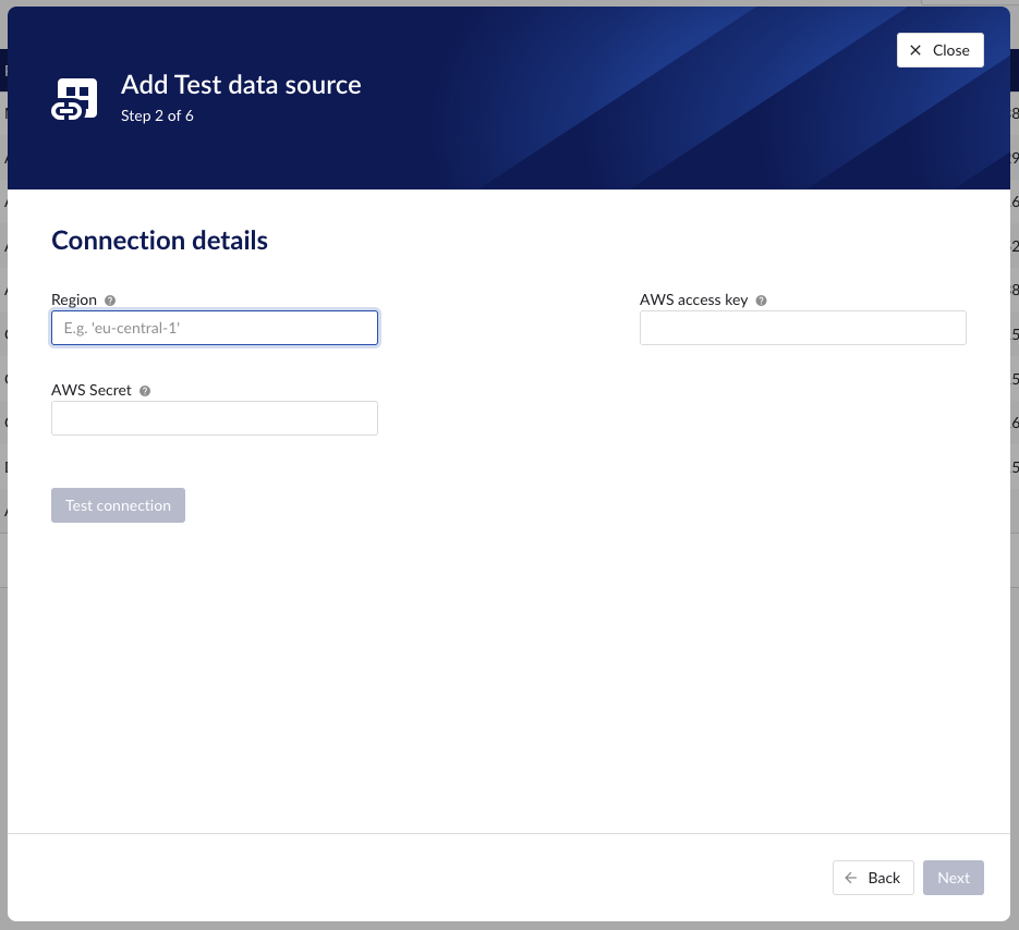
"Region" – enter the availability zone region within AWS cloud in which the AWS IoT SiteWise instance is configured. For more information, please consult the AWS documentation.
"AWS access key" – enter the access key to authenticate. The AWS access key as generated in AWS IAM. For more information, please consult the AWS documentation.
"AWS Secret" – enter the secret to authenticate. The AWS secret as generated in AWS IAM. For more information, please consult the AWS documentation.
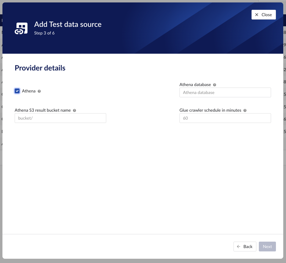
“Athena”
if the Athena option is not enabled, the provider will ingest hot tier data only, using the AWS IoT SiteWise REST API.
if the Athena option is enabled the provider will ingest also cold tier data using Athena queries.
“Athena database” - the name of the Athena database. For more information, please consult the AWS documentation.
“Athena S3 result bucket name” - Athena query results are stored after execution in a S3 result bucket. Specify here the name of the bucket. For more information, please consult the AWS documentation.
“Glue crawler schedule in minutes” - value of Glue crawler interval in minutes. For more information, please consult AWS documentation.
Time series capability
With this capability enabled the datasource can sync Metrics, Transforms and Measurements from AWS IoT SiteWise into TrendMiner tags.
Following properties need to be populated:
“Name“ - а mandatory name needs to be specified.
“Provider” - select the option AWS IoT SiteWise from the dropdown.
“Capabilities” - the AWS IoT SiteWise provider supports the Asset, Time series and Context capabilities.
“Prefix” - optional text can be entered here that will be used to prefix the tag names in TrendMiner, if a value is entered. Warning: this cannot be changed. The datasource can however be deleted and you can start the configuration over again.
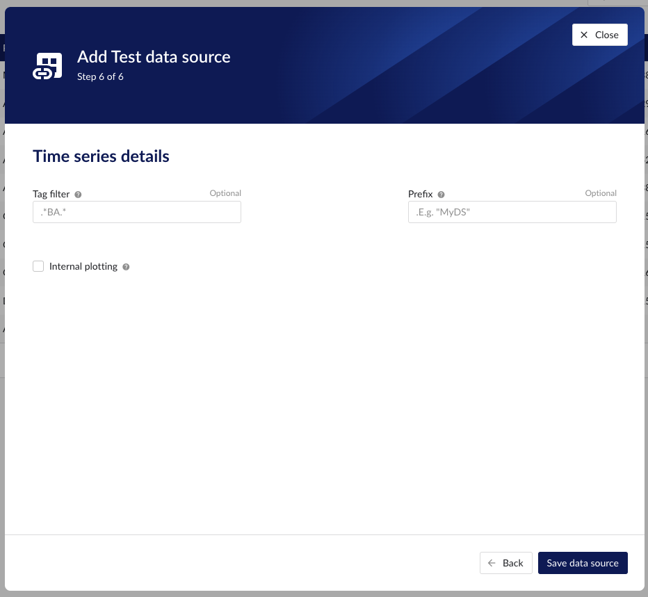
“Tag filter” - an optional regular expression to be entered. Only tags with names that match this regex will be retained when creating tags (using the tag list query).
"Region" – enter the availability zone region within AWS cloud in which the AWS IoT SiteWise instance is configured. For more information, please consult the AWS documentation.
"AWS access key" – enter the access key to authenticate. The AWS access key as generated in AWS IAM. For more information, please consult the AWS documentation.
"AWS Secret" – enter the secret to authenticate. The AWS secret as generated in AWS IAM. For more information, please consult the AWS documentation.
“Athena”
if the Athena option is not enabled, the provider will ingest hot tier data only, using the AWS IoT SiteWise REST API.
if the Athena option is enabled the provider will ingest also cold tier data using Athena queries.
“Athena database” - the name of the Athena database. For more information, please consult the AWS documentation.
“Athena S3 result bucket name” - Athena query results are stored after execution in a S3 result bucket. Specify here the name of the bucket. For more information, please consult the AWS documentation.
“Glue crawler schedule in minutes” - value of Glue crawler interval in minutes. For more information, please consult AWS documentation.
Context capability
With this capability enabled the datasource can sync Alarms from IoT SiteWise into TrendMiner context items.
Following properties need to be populated:
“Name“ - а mandatory name needs to be specified.
“Provider” - select the option AWS IoT SiteWise from the dropdown.
“Capabilities” - the AWS IoT SiteWise provider supports the Asset, Time series and Context capabilities.
"Region" – enter the availability zone region within AWS cloud in which the AWS IoT SiteWise instance is configured. For more information, please consult the AWS documentation.
"AWS access key" – enter the access key to authenticate. The AWS access key as generated in AWS IAM. For more information, please consult the AWS documentation.
"AWS Secret" – enter the secret to authenticate. The AWS secret as generated in AWS IAM. For more information, please consult the AWS documentation.
Setting up S3, Glue, Athena
The very first thing that needs to be done is the creation of the S3 bucket. To do that, we need to provide the bucket name and the region. There are specific rules about the bucket name which can be found here. You can also refer to the step by step guide to create an S3 bucket.
To be able to read data from S3, the AWS IoT SiteWise storage needs to be enabled with the following configuration:
Left menu → Settings → Storage → Edit storage.
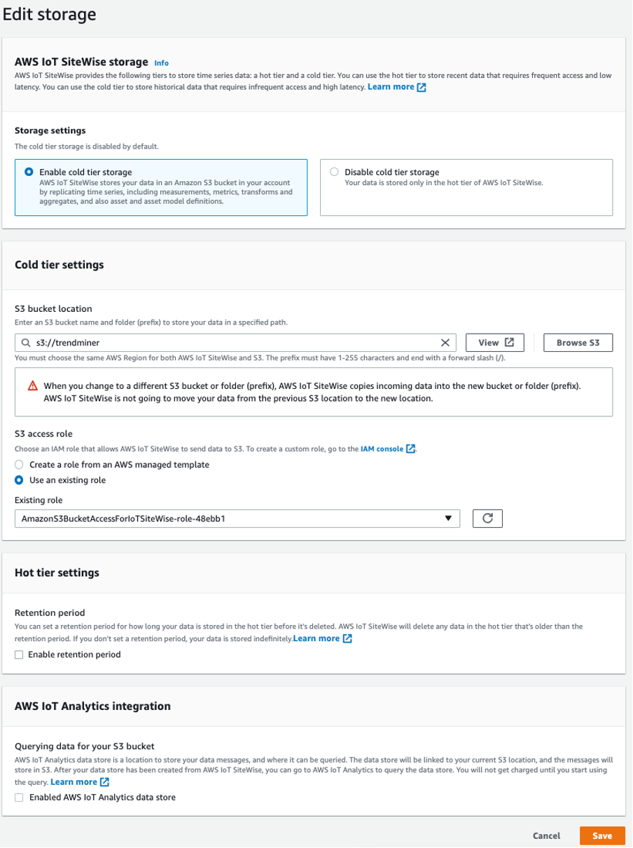
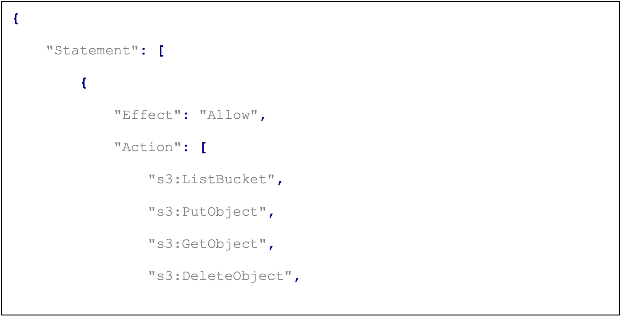
The creation of the role needs the following policies. Pay attention at the bucket name: "arn:aws:s3:::trendminer"
Refer to the AWS documentation on configuring storage settings.
Database creation - not mandatory as a separate step. The name must be unique.
Configuring a crawler:
Example configuration.
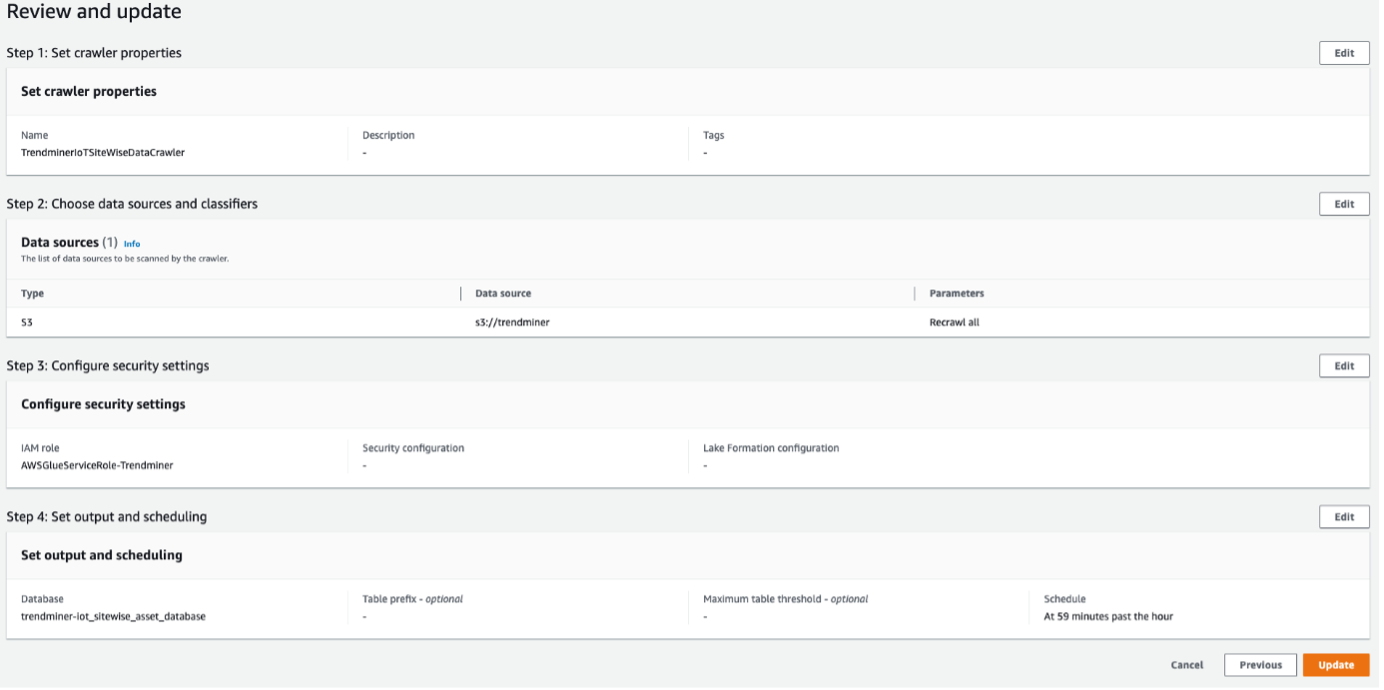
Once the configuration is done, you need to manually Run the crawler. This process might take several minutes, so you should wait until the state becomes Ready.
You can refer to the AWS Documentation on creating a Glue crawler.
Once your crawler status is Ready, you can query your data:
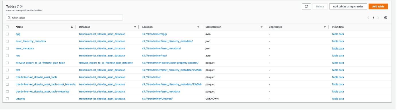
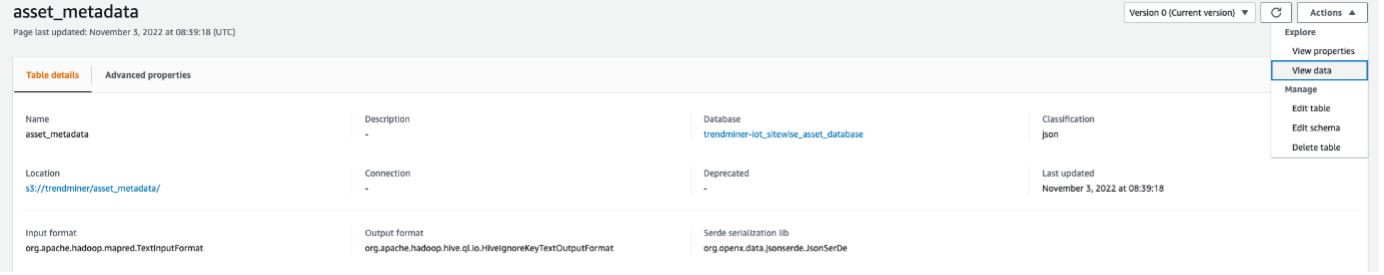
In the navigation pane Data Catalog → Databases → Tables → asset_metadata table of your database and click on the Table data link (more information on how crawlers work - here).
Select the table and continue.
A confirmation pop-up appears. By clicking Proceed you will be automatically redirected to AWS Athena.
Once your crawler runs successfully, you are redirected to AWS Athena:
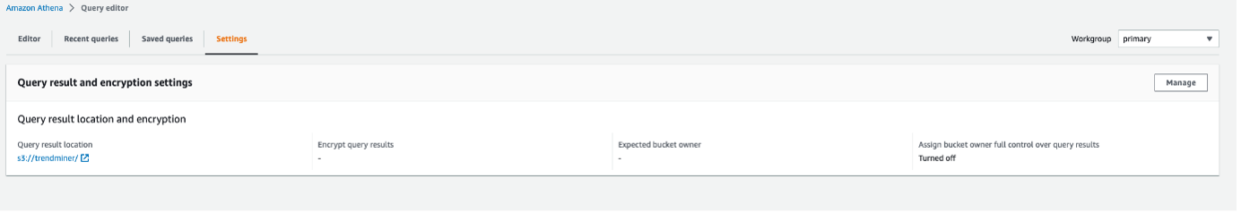
Provide a configuration about the Query result location.
Provide your S3 bucket location.
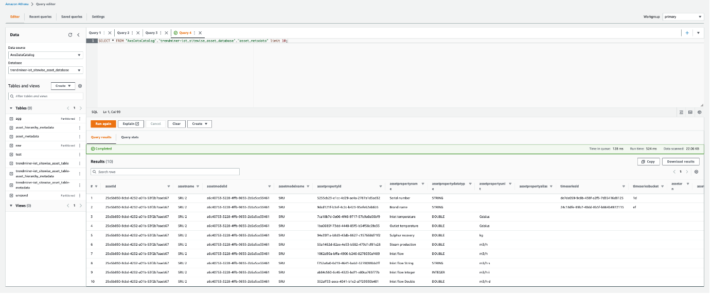
A query can be executed now.
Refer to the AWS Documentation on how to query data with Athena.
How to set up an Amazon Timestream data source?
The following sections will detail all the information needed top set up an Amazon Timestream data source in TrendMiner.
To add an Amazon Timestream data source, in ConfigHub go to Data in the left side menu, then Data sources, choose + Add data source.
Fill out 'Data source details' on the first step of the datasource creation wizard: type name of data source, select “Amazon Timestream” from the Provider dropdown. Time series capability will be checked by default.
Fill out additional properties, grouped in following sections:
Connection details – lists properties related to the configuration of the connection that will be established with Amazon Timestream.
Time series details – lists properties relevant for the time series data.
Following properties need to be populated to establish the connection:
“Prefix” - optional text can be entered here that will be used to prefix the tag names in TrendMiner, if a value is entered. Warning: this cannot be changed. The datasource can however be deleted and you can start the configuration over again.
"Region" – enter the availability zone region within AWS cloud in which the Amazon Timestream instance is configured. For more information, please consult the AWS Documentation.
"AWS access key" – enter the access key to authenticate. This is the access key id as created in AWS IAM.
"AWS Secret" – enter the secret to authenticate. This is the AWS secret as created in AWS IAM.
“Database” – enter the name of database in Amazon Timestream. This is primarily used to test the connection liveness from TrendMiner to Amazon Timestream.
“Tag list query” - a query used by TrendMiner to create tags. A query needs to be provided that given the database schema and tables used will return the following columns:
id - this is mandatory and must have a unique value for each row returned by the query.
name - this is mandatory and must have a value.
type - an optional type indication. If the type column is not in the query, TrendMiner will use the default type which is ANALOG. Custom types can be returned here not known to TrendMiner but then a type mapping must be added as well. See also type mapping below. Without additional type mapping it must be one of the following TrendMiner tag types: ANALOG, DIGITAL, DISCRETE, STRING
description - an optional description to describe the tag. Can return an empty value or null.
units - an optional indication of the units of measurement for this tag. Can return an empty value or null.
The order of the columns in the query needs to be: id, name, type, description, units
“Index query” - a query used by TrendMiner to ingest timeseries data for a specific tag. The query is expected to return a ts (timestamp) and a value. The following variables are available to be used in the WHERE clause of this query. The variables will be substituted at query execution with values. There should not be any NULL values returned by the SELECT statement so including "IS NOT NULL" in the WHERE clause is strongly recommended.
{ID}. The id as returned by the tag list query.
{STARTDATE} TrendMiner will ingest data per intervals of time. This denotes the start of such an interval.
{ENDDATE} TrendMiner will ingest data per intervals of time. This denotes the end of such an interval.
{INTERPOLATION}: Interpolation type of a tag, which can be one of two values: LINEAR or STEPPED.
{INDEXRESOLUTION}: Index resolution in seconds. It can be used to optimise a query to return the expected number of points.
“Digital states query” - if tags of type DIGITAL are returned by the tag list query, TrendMiner will use this query to ask for the {stringValue, intValue} pairs for a specific tag to match a label with a number. The query expects to return a stringValue and an intValue and can make use of the {ID} variable in the where clause. The variable will be substituted at query execution with a value.
“Tag filter” - an optional regular expression to be entered. Only tags with names that match this regex will be retained when creating tags (using the tag list query).
“Type mapping” - if types differ from what TrendMiner uses and one wants to avoid overcomplicating the query, a type mapping can be entered here. It can contain multiple lines and expect per line the value to be representing a custom type followed by a ; and a TrendMiner type. During the execution of the tag list query TrendMiner will then use this mapping to map the custom values returned in the query to TrendMiner tag types.
customTypeA;ANALOG
customTypeB;DIGITAL
customTypeC;DISCRETE
customTypeD;STRING
Example queries
The following exemples are based on the sample data setup in Amazon Timestream – containing a sample database with IoT sample data. Amazon Timestream will then create a sample database that contains IoT sensor data from one or more truck fleets to streamline fleet management and to identify cost optimization opportunities such as reduction in fuel consumption. For more information, please consult https://docs.aws.amazon.com/index.html.
This query treats the location measurements as tags of type STRING.
SELECT distinct
CONCAT(truck_id, '--',measure_name) as id,
CONCAT(truck_id, '--',measure_name) as name,
CASE measure_name
    WHEN 'load' THEN 'DISCRETE'
    WHEN 'location' THEN 'STRING'
    ELSE 'ANALOG'
 END
 AS type,
CONCAT(make, ' ', model, ' (', fleet , ')') AS description,
 CASE measure_name
    WHEN 'load' THEN 'kg'
    WHEN 'speed' THEN 'km/h'
    WHEN 'fuel-reading' THEN '%'
    ELSE ''
 END
 AS unit
FROM sampleDB2.IoT
Alternative query treats the location measurements as tags of type DIGITAL. This is a somewhat less realistic case, but it serves the purpose of also demonstrating tags of type DIGITAL. Location measurements are given a random number between 1 and 10 in the matching alternative index query.
SELECT distinct
CONCAT(truck_id, '--',measure_name) as id,
CONCAT(truck_id, '--',measure_name) as name,
 CASE measure_name
    WHEN 'load' THEN 'DISCRETE'
    WHEN 'location' THEN 'DIGITAL'
    ELSE 'ANALOG'
 END
 AS type,
CONCAT(make, ' ', model, ' (', fleet , ')') AS description,
 CASE measure_name
    WHEN 'load' THEN 'kg'
    WHEN 'speed' THEN 'km/h'
    WHEN 'fuel-reading' THEN '%'
    ELSE ''
 END
 AS unit
FROM sampleDB2.IoT select time as ts,
CASE WHEN measure_value::double is not null
THEN cast(measure_value::double as varchar)
ELSE measure_value::varchar
END AS value
from "sampleDB2"."IoT" where
concat(truck_id, '--',measure_name) = '{ID}'
and time >= '{STARTDATE}'
and time <= '{ENDDATE}'
order by time ascAlternative index query for digital location tags. Where we for the purpose of this demo case assign a random number to a location value for a timestamp.
select time as ts,
CASE SPLIT('{ID}', '--')[2]
    WHEN 'location' THEN RANDOM(10)
    ELSE "measure_value::double"
END AS value
from "sampleDB2"."IoT" where
 concat(truck_id, '--',measure_name) = '{ID}'
 and time >= '{STARTDATE}'
 and time <= '{ENDDATE}'
order by time ascThis query is applicable when the alternative tag list and alternative index query is used.
SELECT 'STATE0' as stringValue, 0 as intValue UNION
SELECT 'STATE1', 1 UNION
SELECT 'STATE2', 2 UNION
SELECT 'STATE3', 3 UNION
SELECT 'STATE4', 4 UNION
SELECT 'STATE5', 5 UNION
SELECT 'STATE6', 6 UNION
SELECT 'STATE7', 7 UNION
SELECT 'STATE8', 8 UNION
SELECT 'STATE9', 9 UNION
SELECT 'STATE10', 10
ORDER BY 1
How to connect to Aspentech APRM?
Aspen Production Record Manager is an information management system for batch type data. A batch in Production Record Manager is subdivided into subbatches and contains attributes called characteristics.
Characteristics represent most types of attributes, including start and end times, batch header data, units, recipe information, batch end data, and so on. In addition, Production Record Manager can generate certain attributes dynamically, such as tag statistics, when requested. The batches are grouped by area and one or more batch areas exist in a Production Record Manager server.
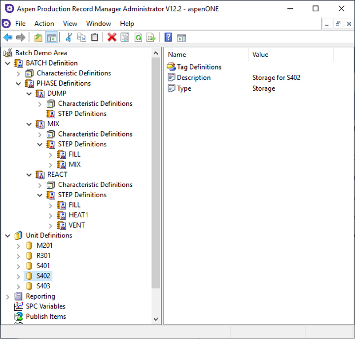
Our provider for Aspen Production Record Manager implements the asset capability and uses data from the area definition to populate the asset hierarchy in TrendMiner. The root node of the asset hierarchy is the area itself. The children nodes of an area node are created using “Unit Definitions". The “Tag Definitions“ are the children of the unit nodes, and the leaf nodes of the asset hierarchy. The asset hierarchy has a fixed depth of two or three.
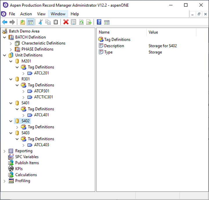
Area, Unit and Tag Definitions in Aspen Production Record Manager Administrator
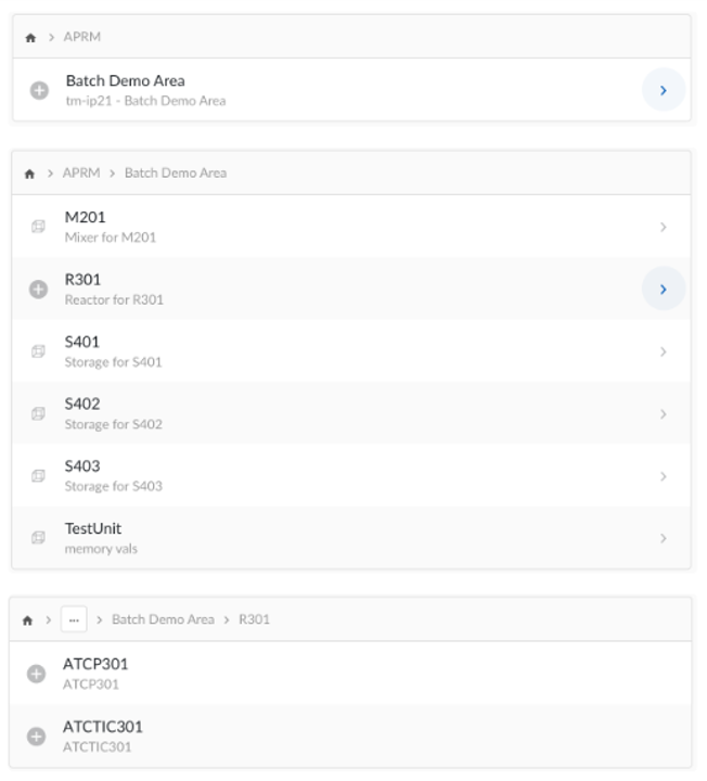
Asset hierarchy in TrendMiner
Our provider for Aspen Production Record Manager also implements the context capability and uses data from the area definition to populate context items in TrendMiner.
Context Item Types
The provider will create Context Item Types for every subbatch definition in the area definition, and that type will be linked to the Context Items.
Components
The link between the asset hierarchy and the context items is established using components in TrendMiner. The provider uses the Unit Characteristic from the subbatches of Aspen Production Record Manager to determine the component of a Context Item. The subbatch level where the Unit Characteristic is defined in Aspen Production Record Manager can be configured by the customer. Since a unit is generally a physical piece of process equipment, every child subbatch of the subbatch level which defines the Unit Characteristic is also conceptually linked to that unit. This is why the following logic is implemented in the provider:
If a unit characteristic is defined on the subbatch level of the subbatch, the context item of this subbatch will be assigned to a component that represents the unit.
If a unit characteristic is defined on a subbatch level lower than the subbatch - lower level means higher in the ancestor hierarchy, the unit characteristic is inherited from the unit of the ancestor.
If a unit characteristic is not defined on a subbatch level lower than the subbatch, the context item will be assigned to a component that represents the area.
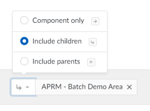
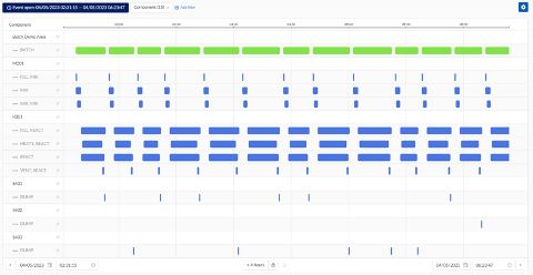
This comes into play when the user starts visualizing multiple subbatch levels at once. Together with the possibility to include the children of a component during filtering it would render the following Gantt, without the users knowing which units belong to the area.
Gantt
Combining the Context Item Types and the implementation of the above component logic, will give the following result in the Gantt view of TrendMiner:
Note
Multiple occurrences of the same subbatches (instances) will be shown in the same swim lane, and the swim lane will be expandable/collapsible.
Context Item properties
The provider generates Context Item properties based on the numeric Characteristics that are available on the subbatches of Aspen Production Record Manager. Only the numeric characteristics are included as Context Item properties, this is by design.
Since numeric characteristics are decimal values in Aspen Production Record Manager, Context Items properties are also formatted decimal numbers.
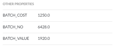
Context item properties
The Start Time, Duration and End Time Characteristics are available as Events. The existence of characteristics and the level on which they are defined is completely dependent on the configuration of the Subbatch Definition implemented on the customer environment.
Multiple occurrences (instances) of the same characteristic can be created during the execution of a subbatch. If a subbatch has multiple instances for a specific characteristic, the characteristics are suffixed with the instance number of the characteristic e.g., BATCH_NO_1 and BATCH_NO_2.
Provider generated property - Lineage
To make the lineage of a context item more apparent, the provider generates the Lineage property, using the same semantics as the Batch Detail Tool.
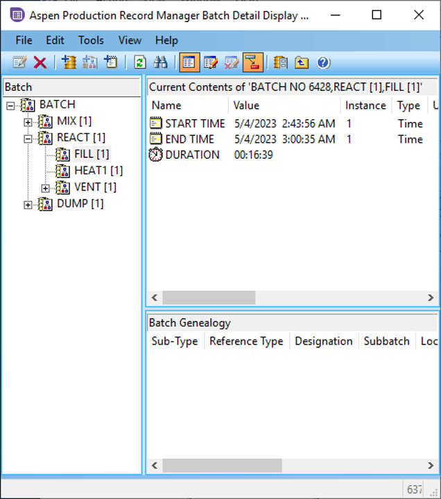
Batch Detail Tool
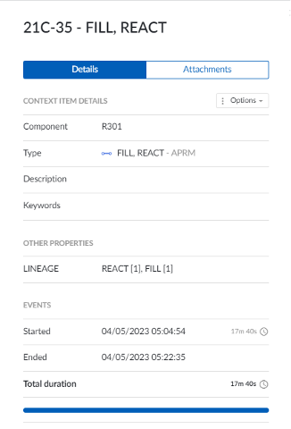
Lineage property in TrendMiner
AtBatch21ApplicationInterface
Our APRM provider uses the AtBatch21ApplicationInterface library which is a component of the AspenONE Manufacturing Execution Systems. This library is installed when you install the Aspen Production Record Manager Server. If Plant Integrations is deployed on the same server, no additional software / configuration is required to use the provider. If it is required to install Plant Integrations of a different server, the Aspen Desktop Application must be installed on the Plant Integrations Service.
Make sure you select the following components from the AspenOne Manufacturing Execution Systems-installer from AspenTech:
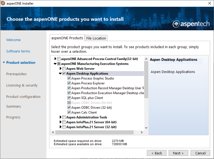
Installing the Aspen Desktop Applications
Important
Because the library uses DCOM, the connector server (Plant Integrations) MUST be in the same domain as the Aspen Production Record Manager server.
Connector (Plant Integrations)
Plant Integrations must be configured to run under an identity that has access to Aspen Production Record Manager. This user must be a member of the 'Distributed COM Users ’group on Aspen Production Record Manager server.
Firewall
If a customer uses a firewall between Plant Integrations and the Aspen Production Record Manager Server, additional ports must be open to allow the DCOM library to communicate with the server.
In ConfigHub go to Data in the left side menu, then Data sources, choose + Add data source. Fill out 'Data source details' on the first step of datasource creation wizard: type the name of a data source, select “Aspen Production Record Manager (via SDK)" from Provider dropdown, then select the configured connector from Connect via dropdown.
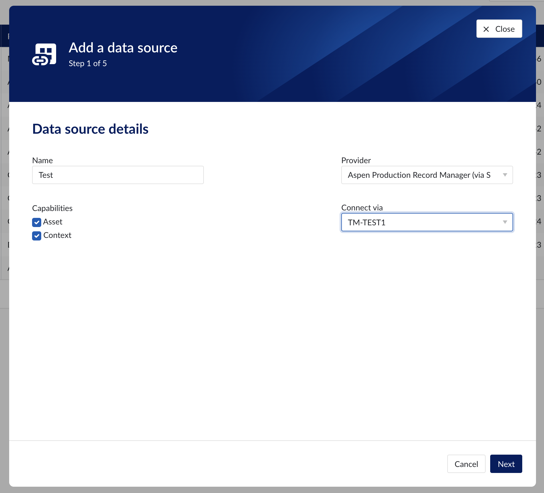
Data source details step in creation wizard
Connection details
To establish a connection 2 optional properties to be filled in:
Property | Description |
|---|---|
Username | Optional convenience field to enter the username used to establish a database connection. As an alternative this information can be entered through the driver properties. |
Password | Optional convenience field to enter the password used to establish a database connection. As an alternative this information can be entered through the driver properties. |
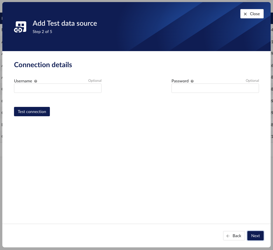
Connection details step in datasource creation wizard
Provider details
The APRM provider implements both assets and context capability. These capabilities have two required provider properties to be filled in:
Property | Description |
|---|---|
Area | The name of the area inside the specified DataSource where the provider reads its data. |
DataSource | The data source used by this provider. The AspenTech Production Record Manager can store multiple data sources on one server instance. |
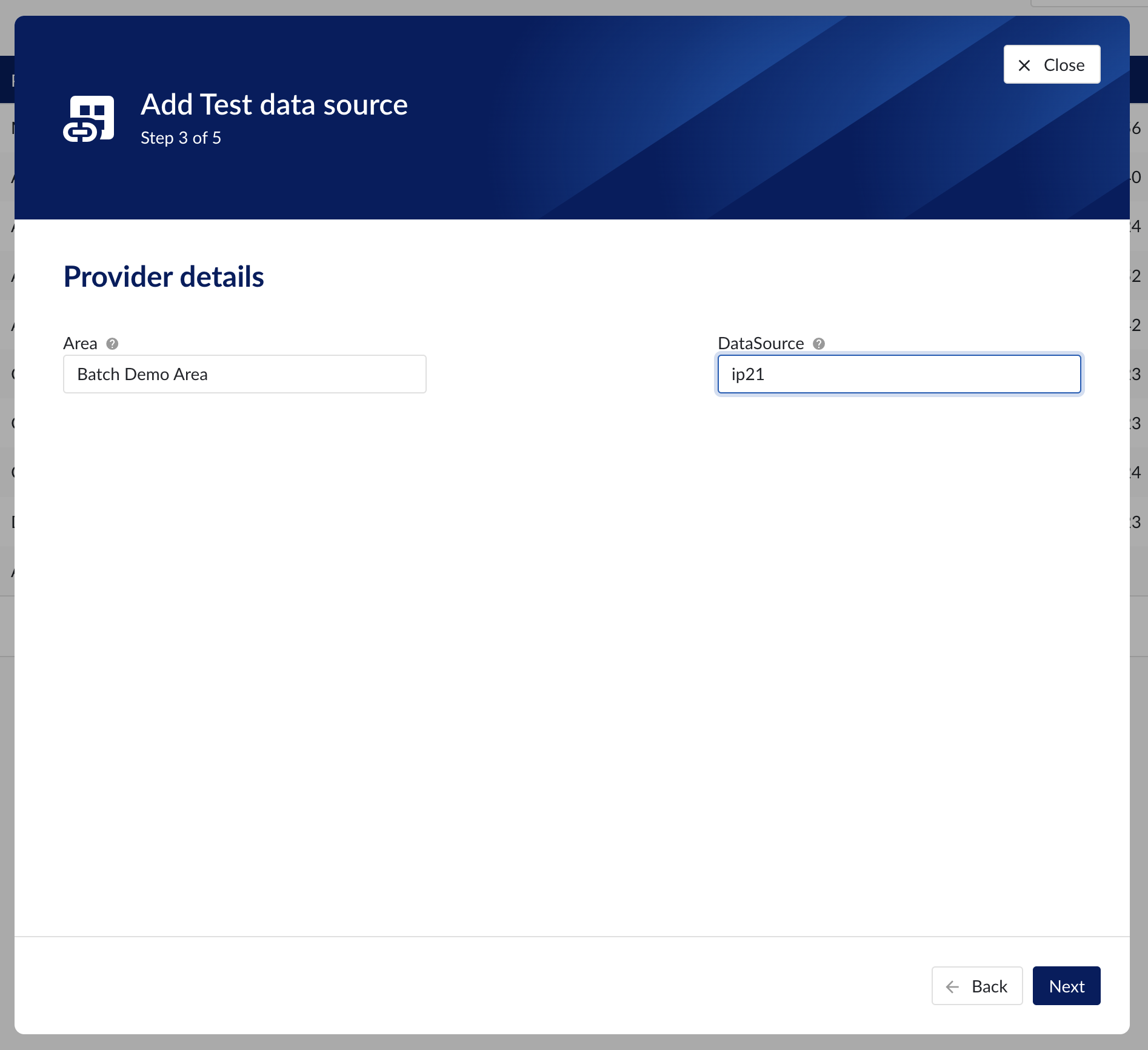
Provider details step in datasource creation wizard
The following are the optional context properties:
Property | Description |
|---|---|
NumberOfSubbatchLevels | Override the number of subbatches to read from the area.This must be a number between (inclusive) 1 and 5. By leaving this property empty, all the levels defined in the area are included (APRM has a limit of 5 levels). |
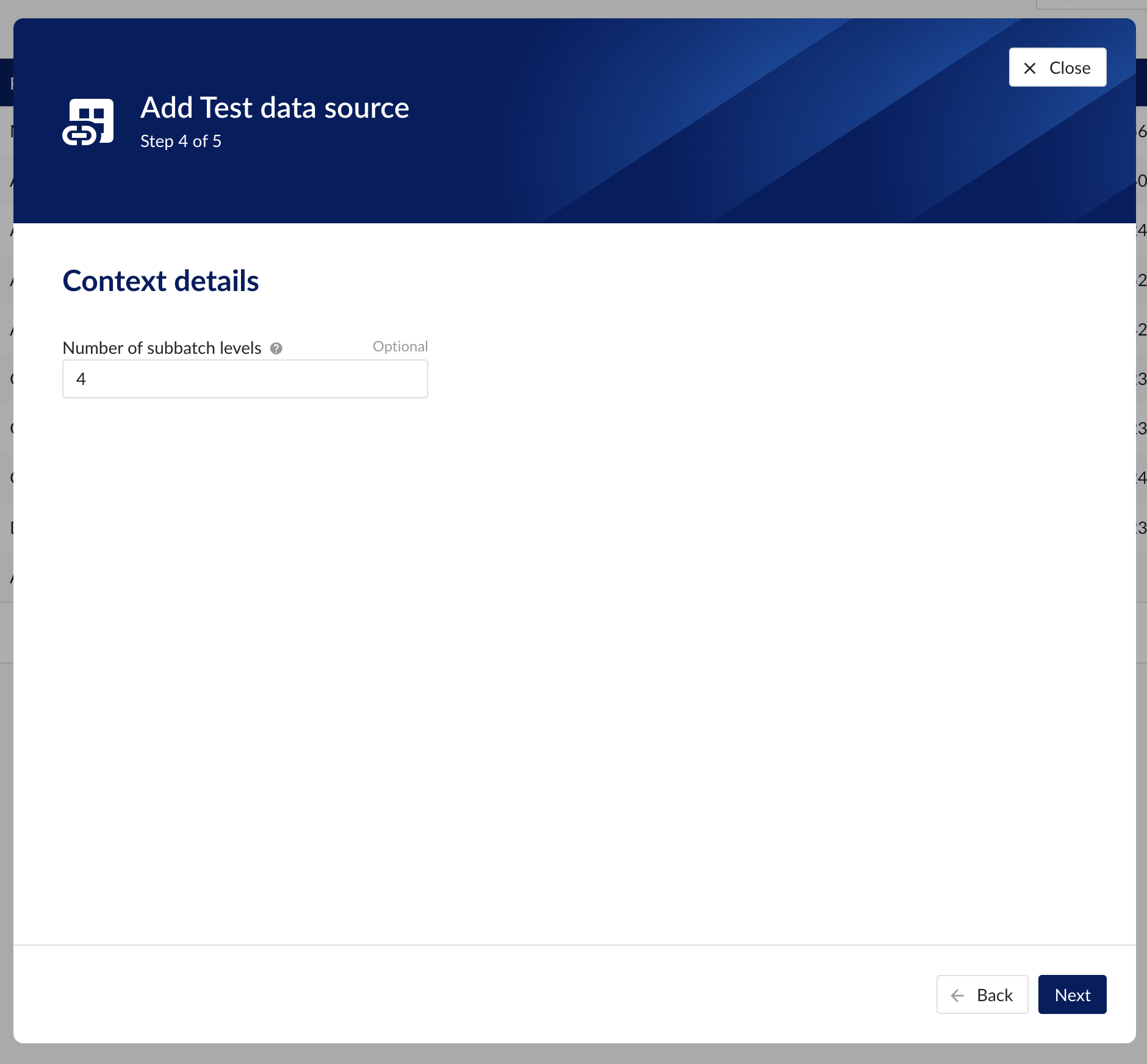
Context details step in datasource creation wizard
Supported versions: 12.2
Interrupt and Resume characteristics are not supported / ignored by the provider.
Planned Start Time and Planned End Time are not supported / ignored by the provider.
How to set up a Generic JDBC data source?
Creating Generic JDBC provider
To integrate with and ingest data from a database that supports JDBC, a datasource of provider type Generic JDBC can be added and configured in ConfigHub.
To add a Generic JDBC data source, in ConfigHub go to Data in the left side menu, then Data sources, choose + Add data source. Fill out 'Data source details' on the first step of the datasource creation wizard: type the name of the data source, select “Generic JDBC” from the Provider dropdown. Selecting the capabilities for the data source with the given checkboxes will open additional properties to enter, grouped in following sections:
Connection details - lists properties related to the configuration of the connection that will be established with datasource
Provider details - lists properties shared by multiple capabilities
Time series details – lists properties relevant for the time series data
Asset details - lists properties relevant for asset data
Context details - lists properties relevant for context data
Following properties need to be populated to establish the connection to the JDBC provider:
“Name“ - а mandatory name needs to be specified.
"Provider" - select the option "Generic JDBC" from the dropdown.
"Capabilities" - the Generic JDBC provider supports the Time series, Asset and Context capabilities.
“Prefix” - optional text can be entered here that will be used to prefix the tag names in TrendMiner, if a value is entered. Warning: this cannot be changed. The datasource can however be deleted and you can start the configuration over again.
"JDBC url" - a mandatory JDBC url to establish a connection to.
"Driver properties" - additional optional driver specific properties can be configured here as key;value, where key is the name of driver specific property and value the desired value for this property. Please consult the documentation of the specific JDBC driver for more information.
"Username" - optional convenience field to enter the username used to establish a database connection. As an alternative this information can be entered through the driver properties.
"Password" - optional convenience field to enter the password used to establish a database connection. As an alternative this information can be entered through the driver properties.
Following properties are shared by multiple capabilities:
"Delimiter" - optional delimiter override, used to parse data values of type STRING_ARRAY. The default is a comma (,)."Delimiter" - optional delimiter override, used to parse data values of type STRING_ARRAY. The default is a comma (,)
Following properties need to be entered to enable time series capability:
“Tag list query” - a query used by TrendMiner to create tags. A query needs to be provided that given the database schema and tables used will return the following columns:
id - this is mandatory and must have a unique value for each row returned by the query.
name - this is mandatory and must have a value.
type - an optional type indication. If the type column is not in the query, TrendMiner will use the default type which is ANALOG. Custom types can be returned here not known to TrendMiner but then a type mapping must be added as well. See also type mapping below. Without additional type mapping it must be one of the following TrendMiner tag types: ANALOG, DIGITAL, DISCRETE, STRING
description - an optional description to describe the tag. Can return an empty value or null.
units - an optional indication of the units of measurement for this tag. Can return an empty value or null.
“Index query” - a query used by TrendMiner to ingest timeseries data for a specific tag. The query is expected to return a ts (timestamp) and a value. The following variables are available to be used in the WHERE clause of this query. The variables will be substituted at query execution with values. There should not be any NULL values returned by the SELECT statement so including "IS NOT NULL" in the WHERE clause is strongly recommended.
{ID}. The id as returned by the tag list query.
{STARTDATE} TrendMiner will ingest data per intervals of time. This denotes the start of such an interval.
{ENDDATE} TrendMiner will ingest data per intervals of time. This denotes the end of such an interval.
{INTERPOLATION}: Interpolation type of a tag, which can be one of two values: LINEAR or STEPPED.
{INDEXRESOLUTION}: Index resolution in seconds. It can be used to optimise a query to return the expected number of points.
“Internal plotting” - if this option is selected TrendMiner will use interpolation if needed to plot the timeseries on the chart on specific time ranges. If this value is not selected and no plot query was provided, TrendMiner will plot directly from the index.
“Plot query” – a query used by TrendMiner to plot timeseries data for a specific tag. The query is expected to return a ts (timestamp) and a value. The following variables are available to be used in the WHERE clause of this query. The variables will be substituted at query execution with values. There should not be any NULL values returned by the SELECT statement so including "IS NOT NULL" in the WHERE clause is strongly recommended.
{ID}. The id as returned by the tag list query.
{STARTDATE}. TrendMiner will plot data per intervals of time. This denotes the start of such an interval.
{ENDDATE}. TrendMiner will plot data per intervals of time. This denotes the end of such an interval.
{INTERPOLATION}: Interpolation type of a tag, which can be one of two values: LINEAR or STEPPED.
{INDEXRESOLUTION}: Index resolution in seconds. It can be used to optimise a query to return the expected number of points.
“Digital states query” - if tags of type DIGITAL are returned by the tag list query, TrendMiner will use this query to ask for the {stringValue, intValue} pairs for a specific tag to match a label with a number. The query expects to return a stringValue and an intValue and can make use of the {ID} variable in the where clause. The variable will be substituted at query execution with a value.
“Tag filter” - an optional regular expression to be entered. Only tags with names that match this regex will be retained when creating tags (using the tag list query).
“Type mapping” - if types differ from what TrendMiner uses and one wants to avoid overcomplicating the query, a type mapping can be entered here. It can contain multiple lines and expect per line the value to be representing a custom type followed by a ; and a TrendMiner type. During the execution of the tag list query TrendMiner will then use this mapping to map the custom values returned in the query to TrendMiner tag types.
customTypeA;ANALOG
customTypeB;DIGITAL
customTypeC;DISCRETE
customTypeD;STRING
"Datetime format" - optional format your time series data are stored in.
"Timezone" – optional timezone your times series data are stored in. Default is "UTC". The format of the timezone is as defined in the IANA time zone database. Valid timezone examples are:
"Europe/Brussels"
"America/Chicago"
"Asia/Kuala_Lumpur"
Following properties need to be entered to enable asset capability:
"Root asset query" - this query is responsible for returning all top level elements from the asset tree structure. It will be used to traverse further down the tree using to queries below. The order of the columns in the result needs to be:
id. Required, unique identifier for this asset record.
type. Required, TrendMiner can handle asset of type ASSET or ATTRIBUTE. This column must be one of these two values.
name. Required, name for this asset record.
description. Optional, description for this asset record.
data type. Optional, TrendMiner can ingest 4 different types of data in case the asset is of type ATTRIBUTE. This column will impact on how the data value column will be interpreted:
STRING data value is interpreted as text
STRING_ARRAY comma delimited string
NUMERIC
DATA_REFERENCE
data value. Optional, this column will either be interpreted as text (STRING), a collection of text (STRING_ARRAY), a number (NUMERIC), or a reference to a tag (DATA_REFERENCE).
"Asset query" - this query returns details for a specific asset record. The following variables are available to be used in the where clause of this query. The variables will be substituted at query execution with values:
{ID}. The id as the unique asset identification.
The order of the columns in the result needs to be:
id. Required, unique identifier for this asset record.
type. Required, TrendMiner can handle asset of type ASSET or ATTRIBUTE. This column must be one of these two values.
name. Required, name for this asset record.
description. Optional, description for this asset record.
data type. Optional, TrendMiner can ingest 4 different types of data in case the asset is of type ATTRIBUTE. This column will impact on how the data value column will be interpreted:
STRING data value is interpreted as text
STRING_ARRAY comma delimited string
NUMERIC
DATA_REFERENCE
data value. Optional, this column will either be interpreted as text (STRING), a collection of text (STRING_ARRAY), a number (NUMERIC), or a reference to a tag (DATA_REFERENCE).
"Asset children query" - this query returns the ids of the direct descendants of the asset. The id passed is the parent, the records returned are its child nodes. The following variables are available to be used in the where clause of this query. The variables will be substituted at query execution with values:
{ID}. The id as the unique asset identification.
The order of the columns in the result needs to be:
id. Required, unique identifier for this asset record.
Following properties need to be entered to enable context capability:
"Events query" - this query is responsible for returning events from the source database. Context items will be generated based on these events.
{AFTER}and{BEFORE}placeholders can be used in the query. They will be replaced with values received in the API call. AdditionalEvent fields querywill be executed to populate custom field values for a specific event. The order of the columns in the result needs to be:id. Required, unique identifier for this event record.
name. Required, name for this event record.
type. Required, event type id. Full information about event type will be fetched in
Type by id query.occurred_at. Required, timestamp when the event has occurred.
modified_at. Required, timestamp when the event was modified.
components. Required, list of component (asset) ids separated by the Delimiter (',' by default).
state. Optional, state for this event record.
description. Optional, description for this event record.
keywords. Optional, list of keywords separated by the Delimiter (',' by default).
"Event by id query" - this query is responsible for returning a specific event from the source database.
{ID}placeholder can be used in the query. It will be replaced with the value received in the API call. AdditionalEvent fields querywill be executed to populate custom field values for specific event. The order of the columns in the result needs to be:id. Required, unique identifier for this event record.
name. Required, name for this event record.
type. Required, event type id. Full information about event type will be fetched in
Type by id query.occured_at. Required, timestamp when the event has occurred.
modified_at. Required, timestamp when the event was modified.
components. Required, list of component (asset) ids separated by the Delimiter (',' by default).
state. Optional, state for this event record.
description. Optional, description for this event record.
keywords. Optional, list of keywords separated by the Delimiter (',' by default).
"Types query" - this query is responsible for returning a list of possible event types from the source database. The order of the columns in the result needs to be:
id. Required, unique identifier for this event record.
name. Required, name for this event record.
color. Optional, color for this event type record. It will be used in the Gantt chart view of the ContextHub.
startstate. Optional, name of the start state.
endstate. Optional, name of the end state.
states. Optional, list of possible states separated by the Delimiter (',' by default).
fields. Optional, list of custom field definition ids for this event record separated by the Delimiter (',' by default).
"Type by id query" - this query is responsible for returning an event type from the source database.
{ID}placeholder can be used in the query. It will be replaced with the value received in the API call. The order of the columns in the result needs to be:id. Required, unique identifier for this event record.
name. Required, unique identifier for this event record.
color. Optional, color for this event type record. It will be used in the Gantt chart view of the ContextHub.
startstate. Optional, name of the start state.
endstate. Optional, name of the end state.
states. Optional, list of possible states separated by the Delimiter (',' by default).
fields. Optional, list of custom field definition ids for this event record separated by the Delimiter (',' by default).
"Fields query" - this query is responsible for returning a list of possible custom fields from the source database. The order of the columns in the result needs to be:
id. Required, unique identifier for this field record.
name. Required, name for this field record.
type. Required, possible values:
STRING
NUMERIC
ENUMERATION
placeholder. Optional, placeholder will be displayed in the ContextHub event creation form.
options. Optional, if type is
ENUMERATIONthis value is required. A list of possible values separated by the Delimiter (',' by default).
"Field by id query" - this query is responsible for returning a custom field from the source database.
{ID}placeholder can be used in the query. It will be replaced with the value received in the API call. The order of the columns in the result needs to be:id. Required, unique identifier for this field record.
name. Required, name for this field record.
type. Required, possible values:
STRING
NUMERIC
ENUMERATION
placeholder. Optional, placeholder will be displayed in the ContextHub event creation form.
options. Optional, if type is
ENUMERATIONthis value is required. A list of possible values separated by the Delimiter (',' by default).
"Event fields query" - this query is responsible for returning custom field values for specific event.
{ID}placeholder can be used in the query. It represents an event id and will be replaced with the value received in the API call. The order of the columns in the result needs to be:fieldId. Required, unique identifier of custom field definition (provided in the Fields query).
value. Required, field value.
"Events Sort column" - column name that will be used for sorting and paging of the events. If value is not set, "id” column will be used by default.
"Events sort column DataType" - the data type of Events sort column. Possible values are: Text, Numeric, DateTime. If value is not set, 'Text' value will be used by default.
"Events id column DataType" - the data type of Events id column (used in Event by id query). Possible values are: Text, Numeric, DateTime. If value is not set, 'Text' value will be used by default.
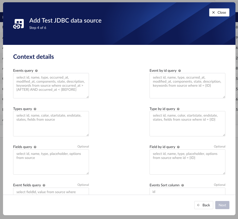
Time series capability
Tag list query
select id, name, type, description, units from source
Index query
select ts, value from source where id={ID} and ts between TO_TIMESTAMP({STARTDATE}, 'YYYY/MM/DD HH24:MI:SS') and TO_TIMESTAMP({ENDDATE}, 'YYYY/MM/DD HH24:MI:SS') and value IS NOT NULL order by ts ascPlot query
select ts, value from source where id={ID} and ts between TO_TIMESTAMP({STARTDATE}, 'YYYY/MM/DD HH24:MI:SS') and TO_TIMESTAMP({ENDDATE}, 'YYYY/MM/DD HH24:MI:SS') and value IS NOT NULL o rder by ts ascDigital states query
This query is applicable when there are tags of type STRING returned through the tag list query.
select stringValue, intValue from source where id={ID}Asset capability
Root asset query
select id, type, name, parentId, description, dataType, dataValue from source where parentId is NULL
Asset query
select id, type, name, description, dataType, dataValue from source where id in ({IDS})Asset children query
select id from source where parentId={ID}Context capability
Events query
select id, name, type, occurred_at, modified_at, components, state, description, keywords from source where occurred_at > TO_TIMESTAMP({AFTER}, 'YYYY/MM/DD HH24:MI:SS') and occurred_at < TO_TIMESTAMP({BEFORE}, 'YYYY/MM/DD HH24:MI:SS')Event by id query
select id, name, type, occurred_at, modified_at, components, state, description, keywords from source where id = {ID}Event types query
select id, name, color, startstate, endstate, states, fields from source
Event type by id query
select id,name, color, startstate, endstate, states, fields from source where id = {ID}Fields query
select id, name, type, placeholder, options from source
Field by id query
select id, name, type, placeholder, options from source where id = {ID}Event fields linked to event query
select fieldId, value from source where eventId = {ID}Time series capability
Tag list query
select id, name, type, description, units from source
Index query
select ts, value from source where id={ID} and ts >= STR_TO_DATE({STARTDATE}, '%Y-%m-%d %H:%i:%S') and ts <=STR_TO_DATE({ENDDATE}, '%Y-%m-%d %H:%i:%S') order by ts ascPlot query
select ts, value from source where id={ID} and ts >= STR_TO_DATE({STARTDATE}, '%Y-%m-%d %H:%i:%S') and ts <=STR_TO_DATE({ENDDATE}, '%Y-%m-%d %H:%i:%S') order by ts ascDigital states query
This query is applicable when there are tags of type STRING returned through the tag list query.
Select stringValue, intValue from source where id={ID}Asset capability
Root asset query
select id, type, name, parentId, description, dataType, dataValue from source where parentId is NULL
Asset query
select id, type, name,description, dataType, dataValue from source where id in ({IDS})Asset children query
select id from source where parentId={ID}Context capability
Events query
select id, name, type, occurred_at, modified_at, components, state, description, keywords from source where occurred_at > STR_TO_DATE({AFTER}, '%Y-%m-%d %H:%i:%S') and occurred_at < STR_TO_DATE({BEFORE}, '%Y-%m-%d %H:%i:%S')Event by id query
select id, name, type, occurred_at, modified_at, components, state, description, keywords from source where id = {ID}Event types query
select id, name, color, startstate, endstate, states, fields from source
Event type by id query
select id,name, color, startstate, endstate, states, fields from source where id = {ID}Fields query
select id, name, type, placeholder, options from source
Field by id query
select id, name, type, placeholder, options from source where id = {ID}Event fields linked to event query
select fieldId, value from source where eventId = {ID}Time series capability
Tag list query
select id, name, type, description, units from source
Index query
select ts, value from source where id={ID} and ts>={STARTDATE} and ts<={ENDDATE} order by ts ascPlot query
select ts, value from source where id={ID} and ts>={STARTDATE} and ts<={ENDDATE} order by ts ascDigital states query
This query is applicable when there are tags of type STRING returned through the tag list query.
select stringValue, intValue from source where id={ID}Asset capability
Root asset query
select id, type, name, parentId, description, dataType, dataValue from source where parentId is NULL
Asset query
select id, type, name, description, dataType, dataValue from source where id in ({IDS})Asset children query
select id from source where parentId={ID}Context capability
Events query
select id, name, type, occurred_at, modified_at, components, state, description, keywords from source where occurred_at >{AFTER} and occurred_at <{BEFORE}Event by id query
select id, name, type, occurred_at, modified_at, components, state, description, keywords from source where id = {ID}Event types query
select id, name, color, startstate, endstate, states, fields from source
Event type by id query
select id,name, color, startstate, endstate, states, fields from source where id = {ID}Fields query
select id, name, type, placeholder, options from source
Field by id query
select id, name, type, placeholder, options from source where id = {ID}Event fields linked to event query
select fieldId, value from source where eventId = {ID} Time series capability
Tag list query
select id, name, type, description, units from source
Index query
select ts, value from source where id={ID} and ts between convert(DATETIME, {STARTDATE}, 127) and convert(DATETIME, {ENDDATE}, 127) order by ts ascPlot query
select ts, value from source where id={ID} and ts between convert(DATETIME, {STARTDATE}, 127) and convert(DATETIME, {ENDDATE}, 127) order by ts ascDigital states query
This query is applicable when there are tags of type STRING returned through the tag list query.
select stringValue, intValue from source where id={ID}Asset capability
Root asset query
select id, type, name, parentId, description, dataType, dataValue from source where parentId is NULL
Asset query
select id, type, name, description, dataType, dataValue from source where id in ({IDS})Asset children query
select id from source where parentId={ID}Context capability
Events query
select id, name, type, occurred_at, modified_at, components, state, description, keywords from source where occurred_at > {AFTER} and occurred_at < {BEFORE}Event by id query
select id, name, type, occurred_at, modified_at, components, state, description, keywords from source where id = {ID}Event types query
select id, name, color, startstate, endstate, states, fields from source
Event type by id query
select id,name, color, startstate, endstate, states, fields from source where id = {ID}Fields query
select id, name, type, placeholder, options from source
Field by id query
select id, name, type, placeholder, options from source where id = {ID}Event fields linked to event query
select fieldId, value from source where eventId = {ID}