How to set up a Microsoft Azure Data Explorer data source?
The following sections will detail all the information needed for setting up a Microsoft Azure Data Explorer data source in TrendMiner.
Warning
The queries and examples on this page are for illustration only. Adjustments to fit your own specific environment may be required (e.g. matching data types) and fall outside of the scope of this support document.
If you wish to engage for hands-on support in setting up this connection, please reach out to your TrendMiner contact.
Danger
It is not recommended to use the "set notruncation;" option in your queries, as this will remove any restriction in the number of data points returned in each request. In extreme cases, this could cause TrendMiner services to run out of memory. It can be useful to add this option for initial testing, but do not use it in production to avoid sudden issues.
Note that, if a result set is truncated, Azure Data Explorer will return this query as FAILED and plotting/indexing on the TrendMiner side will also fail. This is to avoid working with incomplete data sets. If you run into the truncation limit regularly, it is advised to update your index granularity to a lower value. Also, ensure Analytics Optimization is implemented. An example is included in the next sections.
ConfigHub configuration
To add a Microsoft Azure Data Explorer data source, in ConfigHub go to Data in the left side menu, then Data sources, choose + Add data source.
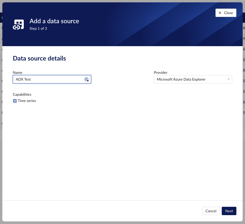
Fill out 'Data source details' on the first step of the datasource creation wizard: type name of data source, select “Microsoft Azure Data Explorer” from the Provider dropdown. Time series capability will be checked by default.
Fill out additional properties, grouped in following sections:
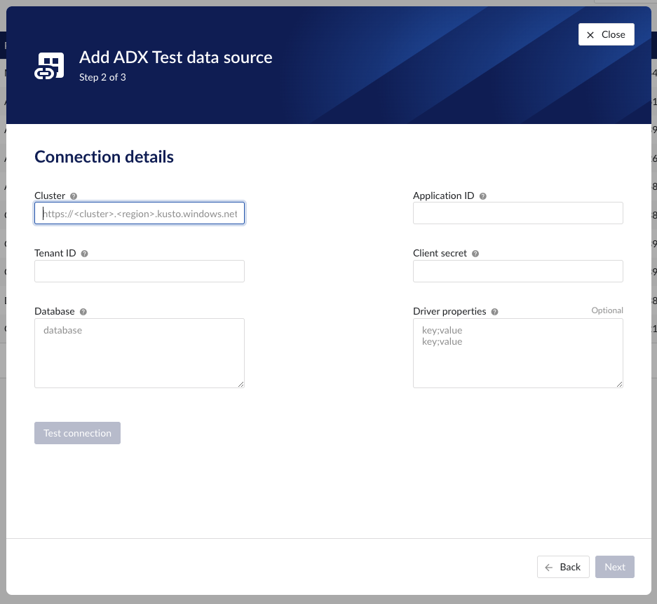
Connection details – lists properties related to the configuration of the connection that will be established with Microsoft Azure Data Explorer.
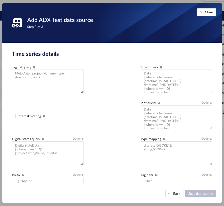
Time series details – lists properties relevant for the time series data.
Following properties need to be populated to establish the connection:
“Name“ - а mandatory name needs to be specified.
“Provider” - select the option Microsoft Azure Data Explorer from the dropdown.
“Capabilities” - the only capability supported is the Time series capability. It will be selected by default.
“Prefix” - optional text can be entered here that will be used to prefix the tag names in TrendMiner, if a value is entered. Warning: this cannot be changed. The datasource can however be deleted and you can start the configuration over again.
"Cluster" - to be mapped with value of the cluster URI.
https://<cluster>.<region>.kusto.windows.net"Application ID" - a mandatory application id. In Azure a new application “TrendMiner” needs to be registered. After completion of this registration the application id will be available. For more info please refer to Azure Active Directory application registration or consult with the Azure Data Explorer documentation.
"Tenant ID" - a mandatory tenant id. In Azure a new application "TrendMiner"needs to be registered. After completion of this registration the tenant id is available.
"Client secret" - after registration of the TrendMiner application in Azure a client id and a secret need to be generated in order to get application access. The client secret for this access needs to be entered here.
"Database" – to be mapped with the name of the ADX database holding the time series data to be pulled.
"Driver properties" - additional optional driver specific properties can be configured here as key;value, where key is the name of driver specific property and value the desired value for this property.
“Tag list query” - a query used by TrendMiner to create tags. A query needs to be provided that given the database schema and tables used will return the following columns:
id - this is mandatory and must have a unique value for each row returned by the query.
name - this is mandatory and must have a value.
type - an optional type indication. If the type column is not in the query, TrendMiner will use the default type which is ANALOG. Custom types can be returned here not known to TrendMiner but then a type mapping must be added as well. See also type mapping below. Without additional type mapping it must be one of the following TrendMiner tag types: ANALOG, DIGITAL, DISCRETE, STRING
description - an optional description to describe the tag. Can return an empty value or null.
units - an optional indication of the units of measurement for this tag. Can return an empty value or null.
The order of the columns in the query needs to be: id, name, type, description, units
“Index query” - a query used by TrendMiner to ingest timeseries data for a specific tag. The query is expected to return a ts (timestamp) and a value. The following variables are available to be used in the WHERE clause of this query. The variables will be substituted at query execution with values.
{ID}. The id as returned by the tag list query.
{STARTDATE} TrendMiner will ingest data per intervals of time. This denotes the start of such an interval.
{ENDDATE} TrendMiner will ingest data per intervals of time. This denotes the end of such an interval.
{INTERPOLATION}: Interpolation type of a tag, which can be one of two values: LINEAR or STEPPED.
{INDEXRESOLUTION}: Index resolution in seconds. It can be used to optimise a query to return the expected number of points.
“Internal plotting” - if this option is selected TrendMiner will use interpolation if needed to plot the timeseries on the chart on specific time ranges. If this value is not selected and no plot query was provided, TrendMiner will plot directly from the index.
“Plot query” – a query used by TrendMiner to plot timeseries data for a specific tag. The query is expected to return a ts (timestamp) and a value. The following variables are available to be used in the WHERE clause of this query. The variables will be substituted at query execution with values.
{ID}. The id as returned by the tag list query.
{STARTDATE}. TrendMiner will plot data per intervals of time. This denotes the start of such an interval.
{ENDDATE}. TrendMiner will plot data per intervals of time. This denotes the end of such an interval.
{INTERPOLATION}: Interpolation type of a tag, which can be one of two values: LINEAR or STEPPED.
{INDEXRESOLUTION}: Index resolution in seconds. It can be used to optimise a query to return the expected number of points.
“Digital states query” - if tags of type DIGITAL are returned by the tag list query, TrendMiner will use this query to ask for the {stringValue, intValue} pairs for a specific tag to match a label with a number. The query expects to return a stringValue and an intValue and can make use of the {ID} variable in the where clause. The variable will be substituted at query execution with a value.
“Tag filter” - an optional regular expression to be entered. Only tags with names that match this regex will be retained when creating tags (using the tag list query).
“Type mapping” - if types differ from what TrendMiner uses and one wants to avoid overcomplicating the query, a type mapping can be entered here. It can contain multiple lines and expect per line the value to be representing a custom type followed by a ; and a TrendMiner type. During the execution of the tag list query TrendMiner will then use this mapping to map the custom values returned in the query to TrendMiner tag types.
customTypeA;ANALOG
customTypeB;DIGITAL
customTypeC;DISCRETE
customTypeD;STRING
Example queries
Example 1 - Minimal configuration
This first example will only implement minimal logic to create a functioning data source. It will not consider Analytics Optimization or implement logic to handle different data types. It is recommended to start with this simple example to ensure the connectivity with ADX is functioning well and to check whether any constraints performance-wise would already pop up. Also, note that ADX will limit the number of output rows. This truncation default is typically 500,000 rows, but can be overridden. If the limit is hit however, ADX will consider this query as FAILED, which causes indexing in TrendMiner to stop.
To create a simple working set of tables with the schemas used in this documentation, the following queries can be executed. Note that this considers data entered as strings in the tables, even though they might represent numeric values (e.g. "5.01").
.create table MetaData (['id']: string, name: string, description: string, ['type']: string, units: string)
.create table Data (['id']: string, ts: datetime, value: string)
.create table DigitalStateData (['id']: string, intValue: long, stringValue: string)
Based on these tables, a tag list query to fetch all tags and their details is a simple project query.
MetaData | project id, name, type, description, units
The index query this simple example selects the data based on the parameters {ID}, {STARTDATE}, and {ENDDATE}. TrendMiner will fill in these variables when sending the query to ADX. Note that this query does not perform any analytics optimization or interpolation. It will simply return all rows that match the conditions. Due to the data schema (the value was defined as string type), this query works for ANALOG, DIGITAL, and STRING tags.
Data
| where ts between (datetime('{STARTDATE}') .. datetime('{ENDDATE}'))
| where id == '{ID}'
| project ts, value| order by ts asc
The plot query will be the same as the index query in this simple example. Once again, all rows that match the conditions will be returned without any further processing.
Data
| where ts between (datetime('{STARTDATE}') .. datetime('{ENDDATE}'))
| where id == '{ID}'
| project ts, value| order by ts asc
To map STRING values to a numeric value (to define the TrendHub y-axis plotting order), the following digital states query can be defined.
DigitalStateData
| where id == '{ID}'
| project stringValue, intValue
Example 2 - Extended configuration
This example will elaborate and will consider different datatypes in the queries and implement the Analytics Optimization. Note that implementing this in the query itself may come with a performance penalty as the logic needs to run when index data is fetched. Especially if the raw data contains many data points, it should be considered whether data can be pre-processed before it is fetched by TrendMiner.
The table schemas for this second example include one table (Data) for tags with decimal values and one table (StringData) for tags with non-decimal values.
.create table MetaData (['id']: string, name: string, description: string, ['type']: string, units: string)
.create table Data (['id']: string, ts: datetime, value: decimal)
.create table StringData ( ts: datetime, id: string, value: string)
.create table DigitalStateData (['id']: string, intValue: long, stringValue: string)
Based on these tables, same as above, a tag list query to fetch all tags and their details is a simple project query.
MetaData | project id, name, type, description, units
The index query in this example is a lot more complete as it handles different scenarios but at the cost of query complexity. Analytics optimization is implemented for numeric tags. This means numeric tags and non-numeric tags need to follow different query paths. This is done by using the union statement near the end of the query, which uses the output of the type filter to query the different tables.
let StringValuesQuery = view() {
    StringData
    | where id == '{ID}'
    | where ts between (datetime('{STARTDATE}') .. datetime('{ENDDATE}'))
    | order by ts asc
    | where isnotempty(value)
    | project ts, value
};
let NumericValuesQuery = view() {
    let _Data = Data
    | where id == '{ID}'
    | where ts between (datetime('{STARTDATE}') .. datetime('{ENDDATE}'))
    | where isnotempty(value)
    | project ts, value
    | order by ts asc;
    let MyTimeline = range ts from datetime('{STARTDATE}') to datetime('{ENDDATE}') step {INDEXRESOLUTION} * 1s;
    MyTimeline
    | union  withsource=source _Data
    | order by ts asc, source asc
    | serialize
    | scan declare (i_min:decimal, i_max:decimal, i_minTs:datetime, i_maxTs:datetime, startValue:decimal, endValue:decimal, startTs:datetime, endTs:datetime, min:decimal, minTs:datetime, max:decimal, maxTs: datetime) with
    (
        step s1 output=none: source=="union_arg0";
        step s2 output=none: source!="union_arg0"=> startValue = iff(isnull(s2.startValue), value, s2.startValue),
                                 startTs = iff(isnull(s2.startTs), ts, s2.startTs),
                                 i_min = iff(isnull(s2.i_min), value, iff(s2.i_min > value, value, s2.i_min)),
                                 i_minTs = iff(isnull(s2.i_min), ts, iff(s2.i_min > value, ts, s2.i_minTs)),
                                 i_max = iff(isnull(s2.i_max), value, iff(s2.i_max < value, value, s2.i_max)),
                                 i_maxTs = iff(isnull(s2.i_max), ts, iff(s2.i_max < value, ts, s2.i_maxTs));
        step s3 output=none: source!="union_arg0" => i_min = iff(isnull(s3.i_min), value, iff(s3.i_min > value, value, s3.i_min)),
                                 i_minTs = iff(isnull(s3.i_min), ts, iff(s3.i_min > value, ts, s3.i_minTs)),
                                 i_max = iff(isnull(s3.i_max), value, iff(s3.i_max < value, value, s3.i_max)),
                                 i_maxTs = iff(isnull(s3.i_max), ts, iff(s3.i_max < value, ts, s3.i_maxTs));
        step s4: source=="union_arg0" => startValue=s2.startValue,
                                     startTs=s2.startTs,
                                     min = s3.i_min,
                                     minTs = s3.i_minTs,
                                     max = s3.i_max,
                                     maxTs = s3.i_maxTs,
                                     endValue= s3.value,
                                     endTs= s3.ts;
    )
    | project startTs, startValue, endTs, endValue, minTs, min, maxTs, max
    | mv-expand     ts  = pack_array(startTs, minTs, maxTs, endTs) to typeof(datetime),
                value = pack_array(startValue, min, max, endValue) to typeof(string)
    | order by ts asc
    | where isnotempty(value)
    | project ts, value
};
let type = toscalar(MetaData
| where id == '{ID}'
| project type);
union (StringValuesQuery() | where tolower(type)=='string'), (NumericValuesQuery() | where not(tolower(type)=='string'))
| where isnotempty(value)
The plot query looks similar conceptually, but just returns raw data so is a lot shorter. Note again the conversion from decimal to string for the NumericValuesQuery to avoid a type mismatch in the union statement.
let StringValuesQuery = view() {
    StringData
    | where id == '{ID}'
    | where ts between (datetime('{STARTDATE}') .. datetime('{ENDDATE}'))
    | order by ts asc
    | where isnotempty(value)
    | project ts, value
};
let NumericValuesQuery = view() {
Data
  | where id == '{ID}'
  | where ts between (datetime('{STARTDATE}') .. datetime('{ENDDATE}'))
  | where isnotempty(value)
  | project ts, value=tostring(value)
  | order by ts asc;
};
let type = toscalar(MetaData
| where id == '{ID}'
| project type);
union (StringValuesQuery() | where tolower(type)=='string'), (NumericValuesQuery() | where not(tolower(type)=='string'))
| where isnotempty(value)